Probability Review

1. Probability Review CS479/679 Pattern RecognitionDr. George Bebis

2. Why Bother About Probabilities? • Probability theory is the proper mechanism for accounting for uncertainty. • Accounting for uncertainty is a crucial component in decision making (e.g., classification) because of ambiguity in our measurements. • Take into account a-priori knowledge, for example: "If the fish was caught in the Atlantic ocean, then it is more likely to be salmon than sea-bass

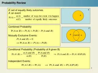
3. Definitions • Random experiment • An experiment whose result is not certain in advance (e.g., throwing a die) • Outcome • The result of a random experiment • Sample space • The set of all possible outcomes (e.g., {1,2,3,4,5,6}) • Event • A subset of the sample space (e.g., obtain an odd number in the experiment of throwing a die = {1,3,5})

4. Intuitive Formulation of Probability • Intuitively, the probability of an event αcould be defined as: • Assumes that all outcomes are equally likely (Laplacian definition) where N(a) is the number of times that eventαhappens in n trials

5. Axioms of Probability S A1 A3 A2 A4 C)

6. Prior (Unconditional) Probability • This is the probability of an event in the absence of any evidence. P(Cavity)=0.1 means that “in the absence of any other information, there is a 10% chance that the patient is having a cavity”.

7. Posterior (Conditional) Probability • This is the probability of an event given some evidence. P(Cavity/Toothache)=0.8 means that “there is an 80% chance that the patient is having a cavity given that he is having a toothache”

8. Posterior (Conditional) Probability (cont’d) • Conditional probabilities can be defined in terms of unconditional probabilities: • Conditional probabilities lead to the chain rule: P(A,B)=P(A/B)P(B)=P(B/A)P(A)

9. Law of Total Probability • If A1, A2, …, An is a partition of mutually exclusive events and B is any event, then: • Special case : S A1 A3 A2 A4

10. Example • My mood can take one of two values: • Happy, Sad • The weather can take one of three values: • Rainy, Sunny, Cloudy • We can compute P(Happy) and P(Sad) as follows: P(Happy)=P(Happy,Rainy)+P(Happy,Sunny)+P(Happy,Cloudy) P(Sad)=P(Sad,Rainy)+P(Sad,Sunny)+P(Sad,Cloudy)

11. Bayes’ Theorem • Conditional probabilities lead to the Bayes’ rule: where

12. Example • Consider the probability of Disease given Symptom:

13. Example (cont’d) • Meningitis causes a stiff neck 50% of the time. • A patient comes in with a stiff neck – what is the probability that he has meningitis? • Need to know the following: • The prior probability of a patient having meningitis (P(M)=1/50,000) • The prior probability of a patient having a stiff neck (P(S)=1/20) P(M/S)=0.0002

14. General Form of Bayes’ Rule • If A1, A2, …, An is a partition of mutually exclusive events and B is any event, then the Bayes’ rule is given by: where

15. Independence • Two events A and B are independent iff: P(A,B)=P(A)P(B) • Using the formula above, we can show: P(A/B)=P(A) and P(B/A)=P(B) • A and B are conditionally independent given C iff: P(A/B,C)=P(A/C) e.g., P(WetGrass/Season,Rain)=P(WetGrass/Rain)

16. Random Variables • In many experiments, it is easier to deal with a summary variable than with the original probability structure. • Example: in an opinion poll, we ask 50 people whether agree or disagree with a certain issue. • Suppose we record a "1" for agree and "0" for disagree. • The sample space for this experiment has 250 elements. • Suppose we are only interested in the number of people who agree. • Define the variable X=number of "1“ 's recorded out of 50. • Easier to deal with this sample space (has only 51 elements).

17. Random Variables (cont’d) • A random variable (r.v.) is a function that assigns a value to the outcome of a random experiment. X(j)

18. Random Variables (cont’d) • How is the probability function of a random variable defined from the probability function of the original sample space? • Suppose the sample space is S=<s1, s2, …, sn> • Suppose the range of the random variable X is <x1,x2,…,xm> • We observe X=xjiff the outcome of the random experiment is an such that X(sj)=xj

19. Example • Consider the experiment of throwing a pair of dice

20. Discrete/Continuous Random Variables • A discrete r.v. can assume only a discrete number of values. • A continuous r.v. can assume a continuous range of values (e.g., sensor readings).

21. Probability mass function (pmf) and probability density function (pdf) • The pmf (discrete r.v.) or pdf (continuous r.v.) of a r.v. X assigns a probability for each possible value of X. • Notation:given two r.v.'s, X and Y, their pmf/pdf are denoted as pX(x) and pY(y); for convenience, we will drop the subscripts and denote them as p(x) and p(y), however, keep in mind that these functions are different!

22. Probability mass function (pmf) and probability density function (pdf) (cont’d) • Some properties of the pmf and pdf:

23. Probability Distribution Function (PDF) • Defined as follows: • Some properties of PDF: • (1) • (2) F(x) is a non-decreasing function of x • If X is discrete, its PDF can be computed as follows:

24. Probability Distribution Function (PDF) (cont’d) pmf

25. Probability Distribution Function (PDF) (cont’d) • If X is continuous, its PDF can be computed as follows: • It can be shown that:

26. Example • Gaussian pdf and PDF 0

27. Joint pmf (discrete r.v.) • For n random variables, the jointpmf assigns a probability for each possible combination of values: p(x1,x2,…,xn)=P(X1=x1, X2=x2, …, Xn=xn) Notation:the joint pmf /pdf of the r.v.'s X1, X2, ..., Xn and Y1, Y2, ..., Yn are denoted as pX1X2...Xn(x1,x2,...,xn) and pY1Y2...Yn(y1,y2,...,yn); for convenience, we will drop the subscripts and denote them p(x1,x2,...,xn) and p(y1,y2,...,yn), keep in mind, however, that these are two different functions.

28. Joint pmf (discrete r.v.) (cont’d) • Specifying the joint pmf requires a large number of values • kn assuming n random variables where each one can assume one of k discrete values. • Can be simplified if we assume independence or conditional independence. P(Cavity, Toothache) is a 2 x 2 matrix Joint Probability Sum of probabilities = 1.0

29. Joint pdf (continuous r.v.) For n random variables, the joint pdf assigns a probability for each possible combination of values:

30. Chain Rule • The conditional pdf can be derived from the joint pdf: • Conditional pdfs lead to the chain rule: • General case:

31. Independence • Knowledge about independence between r.v.'s is very powerful since it simplifies things a lot. e.g., if X and Y are independent, then:

32. Law of Total Probability • The law of total probability:

33. Marginalization • From the joint probability, we can compute the pmf/pdf of any subset of variables by marginalization: • Example (joint pmf) p(x,y): • Examples (joint pdf )p(x,y) : (1) (2) (3)

34. The joint pmf/pdf is very useful!

35. Normal (Gaussian) Distribution dimension d d x 1 d x d symmetric matrix

36. Normal (Gaussian) Distribution (cont’d) • Parameters and shape of Gaussian distribution • Number of parameters is • Shape determined by Σ

37. Normal (Gaussian) Distribution (cont’d) • Mahalanobis distance: • If the variables are independent, the multivariate normal distribution becomes: Σ is diagonal

38. Expected Value

39. Expected Value (cont’d) • The sample mean and expected value are related by: • The expected value for a continuous r.v. is given by:

40. Variance and Standard Deviation

41. Covariance

42. Covariance Matrix Σ = and Cov(X,Y)=Cov(Y,X) (symmetric matrix)

43. Covariance Matrix (cont’d) (symmetric matrix)

44. Uncorrelated r.v.’s

45. Properties of covariance matrix

46. Covariance Matrix Decomposition Φ-1= ΦT

47. Linear Transformations

48. Linear Transformations (cont’d) Whitening transform