Download
1 / 79
790 likes | 916 Vues
This lecture series covers exemplary inverse problems, focusing on theory and applications in tomography and vibrational analysis. Key topics include measurement errors, least squares methods, a priori information, generalized inverses, and techniques like the Backus-Gilbert method. Emphasis is placed on solving complex problems including Earthquake location and vibrational assessments using Fréchet derivatives. Practical methodologies such as the Damped and Weighted Least Squares, along with an introduction to nonlinear problem-solving techniques, are thoroughly explored throughout the lectures.

E N D
Lecture 24 Exemplary Inverse ProblemsincludingVibrational Problems
Syllabus Lecture 01 Describing Inverse ProblemsLecture 02 Probability and Measurement Error, Part 1Lecture 03 Probability and Measurement Error, Part 2 Lecture 04 The L2 Norm and Simple Least SquaresLecture 05 A Priori Information and Weighted Least SquaredLecture 06 Resolution and Generalized Inverses Lecture 07 Backus-Gilbert Inverse and the Trade Off of Resolution and VarianceLecture 08 The Principle of Maximum LikelihoodLecture 09 Inexact TheoriesLecture 10 Nonuniqueness and Localized AveragesLecture 11 Vector Spaces and Singular Value Decomposition Lecture 12 Equality and Inequality ConstraintsLecture 13 L1 , L∞ Norm Problems and Linear ProgrammingLecture 14 Nonlinear Problems: Grid and Monte Carlo Searches Lecture 15 Nonlinear Problems: Newton’s Method Lecture 16 Nonlinear Problems: Simulated Annealing and Bootstrap Confidence Intervals Lecture 17 Factor AnalysisLecture 18 Varimax Factors, Empircal Orthogonal FunctionsLecture 19 Backus-Gilbert Theory for Continuous Problems; Radon’s ProblemLecture 20 Linear Operators and Their AdjointsLecture 21 Fréchet DerivativesLecture 22 Exemplary Inverse Problems, incl. Filter DesignLecture 23 Exemplary Inverse Problems, incl. Earthquake LocationLecture 24 Exemplary Inverse Problems, incl. Vibrational Problems
Purpose of the Lecture • solve a few exemplary inverse problems • tomography • vibrational problems • determining mean directions
Part 1 • tomography
tomography: data is line integral of model function y assume ray path is known ray i x di = ∫ray im(x(s), y(s)) ds
discretization: model function divided up into M pixels mj
data kernelGij= length of ray i in pixel j here’s an easy, approximate way to calculate it
start with G set to zero ray i then consider each ray in sequence
divide each ray into segments of arc length ∆s ∆s and step from segment to segment
determine the pixel index, say j, that the center of each line segment falls within add ∆s to Gij repeat for every segment of every ray
You can make this approximation indefinitely accurate simply bydecreasing the size of ∆s(albeit at the expense of increase the computation time)
Suppose that there are M=L2voxelsA ray passes through about L voxelsG has NL2 elementsNL of which are non-zeroso the fraction of non-zero elements is1/Lhence G is very sparse
In a typical tomographic experimentsome pixels will be missed entirelyand some groups of pixels will be sampled by only one ray
In a typical tomographic experimentsome pixels will be missed entirelyand some groups of pixels will be sampled by only one ray the value of these pixels is completely undetermined only the average value of these pixels is determined hence the problem is mixed-determined (and usually M>N as well)
soyou must introduce some sort of a priori information to achieve a solutionsaya priori information that the solution is smallor a priori information that the solution is smooth
Solution Possibilities • Damped Least Squares (implements smallness): Matrix G is sparse and very large use bicg() with damped least squares function 2. Weighted Least Squares (implements smoothness): Matrix F consists ofG plus second derivative smoothing use bicg()with weighted least squares function
Solution Possibilities • Damped Least Squares: Matrix G is sparse and very large use bicg() with damped least squares function 2. Weighted Least Squares: Matrix F consists ofG plus second derivative smoothing use bicg()with weighted least squares function test case has very good ray coverage, so smoothing probably unnecessary
sources and receivers True model y x
just a “few” rays shown else image is black Ray Coverage y y x x
Data, plotted in Radon-style coordinates distance r of ray to center of image minor data gaps angleθof ray Lesson from Radon’s Problem: Full data coverage need to achieve exact solution
True model Estimated model y x
Estimated model Estimated model y streaks due to minor data gaps they disappear if ray density is doubled x
but what if the observational geometry is poorso that broads swaths of rays are missing ?
complete angular coverage (A) (B) y y x x (C) (D) r y θ x
incomplete angular coverage (A) (B) y y x x (C) (D) r y θ x
Part 2 • vibrational problems
statement of the problem Can you determine the structure of an object just knowing the characteristic frequencies at which it vibrates? frequency
the Fréchet derivativeof frequency with respect to velocity is usually computed using perturbation theoryhence a quick discussion of what that is ...
perturbation theory a technique for computing an approximate solution to a complicated problem, when 1. The complicated problem is related to a simple problem by a small perturbation 2. The solution of the simple problem must be known
Here’s the actual vibrational problemacoustic equation withspatially variable sound velocity v
acoustic equation withspatially variable sound velocity v patterns of vibration or eigenfunctions or modes frequencies of vibration or eigenfrequencies
v(x) = v(0)(x) + εv(1)(x) + ... • assume velocitycan be written as a perturbation • around some simple structure • v(0)(x)
now represent eigenfrequencies and eigenfunctions as power series in ε
now represent eigenfrequencies and eigenfunctions as power series in ε represent first-order perturbed shapes as sum of unperturbed shapes
plug series into original differential equation group terms of equal power of ε solve for first-order perturbation ineigenfrequenciesωn(1) and eigenfunction coefficients bnm • (use orthonormality in process)
result for eigenfrequencies write as standard inverse problem
standard continuousinverse problem perturbation in the eigenfrequencies are the data perturbation in the velocity structure is the model function
standard continuousinverse problem data kernel or Fréchet derivative depends upon the unperturbed velocity structure, the unperturbed eigenfrequency and the unperturbed mode
1D organ pipe open end, p=0 unperturbed problem has constant velocity 0 perturbed problem has variable velocity closed end dp/dx=0 h x
p1 p2 p3 p=0 0 modes h dp/dx=0 x x x x frequencies 𝜔 𝜔1 𝜔2 𝜔3 0