Download
1 / 43
530 likes | 951 Vues
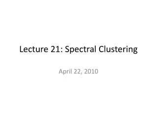
Lecture 21: Spectral Clustering. April 22, 2010. Last Time. GMM Model Adaptation MAP (Maximum A Posteriori) MLLR (Maximum Likelihood Linear Regression) UMB- MAP for speaker recognition. Today. Graph Based Clustering Minimum Cut. Partitional Clustering.

E N D
Lecture 21: Spectral Clustering April 22, 2010
Last Time • GMM Model Adaptation • MAP (Maximum A Posteriori) • MLLR (Maximum Likelihood Linear Regression) • UMB-MAP for speaker recognition
Today • Graph Based Clustering • Minimum Cut
Partitional Clustering • How do we partition a space to make the best clusters? • Proximity to a cluster centroid.
Difficult Clusterings • But some clusterings don’t lend themselves to a “centroid” based definition of a cluster. • Spectral clustering allows us to address these sorts of clusters.
Difficult Clusterings • These kinds of clusters are defined by points that are close any member in the cluster, rather than the average member of the cluster.
Graph Representation • We can represent the relationships between data points in a graph.
Graph Representation • We can represent the relationships between data points in a graph. • Weight the edges by the similarity between points
Representing data in a graph • What is the best way to calculate similarity between two data points? • Distance based:
Graphs • Nodes and Edges • Edges can be directed or undirected • Edges can have weights associated with them • Here the weights correspond to pairwise affinity
Graphs • Degree • Volume of a set
Graph Cuts • The cut between two subgraphs is calculated as follows
Graph Examples - Distance E 4.1 B 5.1 12 1 4.5 2.2 A 11 D 5 C
Graph Examples - Similarity E .24 B .19 .08 1 .22 .45 A .09 D .2 C
Intuition • The minimum cut of a graph identifies an optimal partitioning of the data. • Spectral Clustering • Recursively partition the data set • Identify the minimum cut • Remove edges • Repeat until k clusters are identified
Graph Cuts • Minimum (bipartitional) cut
Graph Cuts • Minimum (bipartitional) cut
Graph Cuts • Minimal (bipartitional) normalized cut. • Unnormalized cuts are attracted to outliers.
Graph definitions • ε-neighborhood graph • Identify a threshold value, ε, and include edges if the affinity between two points is greater than ε. • k-nearest neighbors • Insert edges between a node and its k-nearest neighbors. • Each node will be connected to (at least) k nodes. • Fully connected • Insert an edge between every pair of nodes.
Intuition • The minimum cut of a graph identifies an optimal partitioning of the data. • Spectral Clustering • Recursively partition the data set • Identify the minimum cut • Remove edges • Repeat until k clusters are identified
Spectral Clustering Example • Minimum Cut E .24 B .19 .08 1 .22 .45 A .09 D .2 C
Spectral Clustering Example • Normalized Minimum Cut E .24 B .19 .08 1 .22 .45 A .09 D .2 C
Spectral Clustering Example • Normalized Minimum Cut E .24 B .19 .08 1 .22 .45 A .09 D .2 C
Problem • Identifying a minimum cut is NP-hard. • There are efficient approximations using linear algebra. • Based on the Laplacian Matrix, or graph Laplacian
Spectral Clustering • Construct an affinity matrix A D .2 .2 .1 B C .3
Spectral Clustering • Construct the graph Laplacian • Identify eigenvectors of the affinity matrix
Spectral Clustering • K-Means on eigenvector transformation of the data. • Project back to the initial data representation. k-eigen vectors Each Row represents a data point in the eigenvector space n-data points
Overview: what are we doing? • Define the affinity matrix • Identify eigenvalues and eigenvectors. • K-means of transformed data • Project back to original space
Why does this work? • Ideal Case • What are we optimizing? Why do the eigenvectors of the laplacian include cluster identification information
Why does this work? • How does this eigenvector decomposition address this? • if we let f be eigen vectors of L, then the eigenvalues are the cluster objective functions cluster assignment Cluster objective function – normalized cut!
Normalized Graph Cuts view • Minimal (bipartitional) normalized cut. • Eigenvalues of the laplacianare approximate solutions to mincut problem.
The Laplacian Matrix • L = D-W • Positive semi-definite • The lowest eigenvalue is 0, eigenvector is • The second lowest contains the solution • The corresponding eigenvector contains the cluster indicator for each data point
Using eigenvectors to partition • Each eigenvector partitions the data set into two clusters. • The entry in the second eigenvector determines the first cut. • Subsequent eigenvectors can be used to further partition into more sets.
Example • Dense clusters with some sparse connections
3 class Example Affinity matrix eigenvectors row normalization output
k-means vs. Spectral Clustering K-means Spectral Clustering
Random walk view of clustering • In a random walk, you start at a node, and move to another node with some probability. • The intuition is that if two nodes are in the same cluster, you a randomly walk is likely to reach both points.
Random walk view of clustering • Transition matrix: • The transition probability is related to the weight of given transition and the inverse degree of the currentnode.
Using minimum cut for semi supervised classification? • Construct a graph representation of unseen data. • Insert imaginary nodes s and t connected to labeled points with infinite similarity. • Treat the min cut as a maximum flow problem from s to t t s
Kernel Method • The weight between two nodes is defined as a function of two data points. • Whenever we have this, we can use any valid Kernel.
Today • Graph representations of data sets for clustering • Spectral Clustering
Next Time • Evaluation. • Classification • Clustering