Spectral Clustering
Spectral Clustering. 指導教授 : 王聖智 S . J. Wang 學生 : 羅介暐 Jie -Wei Luo. Outline. Motivation Graph overview Spectral Clustering Another point of view Conclusion. Motivation. K-means performs very poorly in this space due Dataset exhibits complex cluster shapes. K-means.

Spectral Clustering
E N D
Presentation Transcript
Spectral Clustering 指導教授: 王聖智 S. J. Wang 學生:羅介暐 Jie-Wei Luo
Outline • Motivation • Graph overview • Spectral Clustering • Another point of view • Conclusion
Motivation • K-means performs very poorly in this space due Dataset exhibits complex • cluster shapes
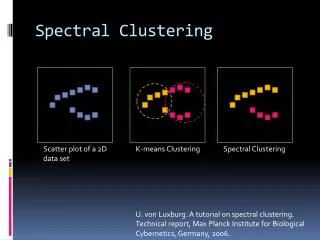
Spectral Clustering Scatter plot of a 2D data set K-means Clustering Spectral Clustering U. von Luxburg. A tutorial on spectral clustering. Technical report, Max Planck Institute for Biological Cybernetics, Germany, 2007.
Graph overview • Graph Partitioning • Graph notation • Graph Cut • Distance and Similarity
Graph partitioning First-graph representation of data Then-graph partitioning In this talk–mainly how to find a good partitioning of a given graph using spectral properties of that graph
Graph notation Always assume that similarities sijare symmetric, non-negative Then graph is undirected, can be weighted Note: 1. Sij0 2. Sij=Sji
Graph notation vi Degree of vertex viє V
Graph Cuts Mincut : min Cut(A1,A2) However, mincut simply seperates one individual vertex from the rest of the graph Balanced cut Problem: finding an optimal graph (normalized) cut is NP-hard Approximation: spectral graph partitioning
Spectral Clustering •Unnormalizedgraph Laplacian • Normalized graph Laplacian • Other explanation • Example
Spectral clustering - main algorithms • Input: Similarity matrix S, number k of clusters to construct • • Build similarity graph • • Compute the first k eigenvectors v1, . . . , vk of the problem matrix • L for unnormalized spectral clustering • Lrw for normalized spectral clustering • • Build the matrix V єRn×k with the eigenvectors as columns • • Interpret the rows of V as new data points ZiєRk • • Cluster the points Zi with the k-means algorithm in Rk
Example-1 W: adjacency matrix D: degree matrix 2 1 3 4 5 Similarity Graph L: Laplacian matrix
Example-1 L: Laplacian matrix 2 1 3 4 First Two Eigenvectors 5 Similarity Graph Double Zero Eigenvalue Two Connected Components v1 v2
Example-1 First k Eigenvectors New Clustering Space 2 1 3 4 5 Use k-means clustering in the new space Similarity Graph v2 v1
Unnormalized graph Laplacian Define as L=D-W proof
Unnormalized graph Laplacian proof • Relation between spectrum and clusters: • Multiplicity of k eigenvalue 0 = number k of connected • components A1, ..., Ak of the graph. • eigenspaceis spanned by the characteristic functions 1A1 , ..., 1Ak • of those components (so all eigenvecotrs are piecewise constant).
Unnormalized graph Laplacian Interpret sij= 1 / d(Xi, Xj )2 looks like a discrete version of the standard Laplace operator
Normalized graph Laplacian Define
Normalized graph Laplacian Spectral properties similar to L: • Positive semi-definite, smallest eigenvalue is 0 • Attention: For Lrw, eigenspace spanned by 1Ai (piecewise const.) but for Lsym, eigenspace spanned by D1/21Ai (not piecewise const).
Random walk explanations General observation: • Random walk on the graph has transition matrix P = D−1W. • note that Lrw = I − P Specific observation about Ncut: • define P(A|B) is the probability to jump from B to A if we assume that the random walk starts in the stationary distribution. • Then: Ncut(A, B) = P(A|B) + P(B|A) • Interpretation: Spectral clustering tries to construct groups such that a random walk stays as long as possible within the same group
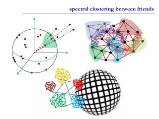
In the embedded space given by two leading eigenvectors, clusters are trivial to separate. Example-2
Example-3 In the embedded space given by three leading eigenvectors, clusters are trivial to separate.
PCA Linear combination the original data Xi to now variable Zi
Rank reduce comparison between PCA & LaplacianEigenmap PCA is linear combination to reduce dimension, though PCA minimize the Reconstruction error, but it’s not helpful to cluster groups. Spectral clustering is nonlinear reducing dimension which is helpful to cluster, however it’s doesn’t actually have a “rank reduce function” apply to new data, while PCA have it.
Conclusion Why is spectral clustering useful? • Does not make strong assumptions on cluster shape • Is simple to implement (solving an eigenproblem) • Spectral clustering objective does not have local optima • Has several different derivations • Successful in many applications What are potential problems? • Can be sensitive to choice of parameters (k in kNN-graph). • Computational expensive on large non-sparse graphs