Download
1 / 14
140 likes | 231 Vues
Learn about spectral clustering techniques with a focus on learning similarity matrices for speech separation applications. This paper introduces cost functions, algorithms, and approximation schemes to optimize clustering results. It discusses traditional techniques, motivations, and new developments in spectral clustering.

E N D
Learning Spectral Clustering, With Application to Speech Separation F. R. Bach and M. I. Jordan, JMLR 2006
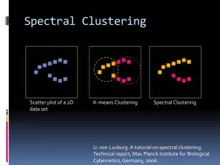
Outline • Introduction • Normalized cuts -> Cost functions for spectral clustering • Learning similarity matrix • Approximate scheme • Examples • Conclusions
Introduction 1/2 • Traditional spectral clustering techniques: • Assume a metric/similarity structure, then use clustering algorithms. • Manual feature selection and weight are time-consuming. • Proposed method • A general framework for learning the similarity matrix for spectral clustering from data. • Assume given data with known partitions and want to build similarity matrices that will lead to these partitions in spectral clustering. • Motivations: • Hand-labelled databases are available: image, speech. • Robust to irrelevant features.
Introduction 2/2 • What’s new? • Two cost functions J1(W, E), J2(W, E), W: similarity matrix, E: a partition. • MinEJ1 New clustering algorithms; • MinW J1 learning the similarity matrix; • W is not necessarily positive semidefinite; • Design numerical approximation scheme for large scale.
Spectral Clustering & NCuts 1/4 • R-way Normalized Cuts • Each data point is one node in a graph, the weight on the edge connecting two nodes is the similarity of those two. • A graph is partitioned into R disjoint clusters by minimizing the normalized cut, cost function, C(A, W), • V={1,…,P}, index set of all data points • A={Ar}rЄ{1,…,R}, Union of Ar=V. • is total weight between A and B. • , normalized term penalizes unbalanced partition.
Spectral Clustering & NCuts 2/4 • Another form of Ncuts: • E=(e1,…,eR), er is the indicator vector (P by 1) for the r-th cluster. • Spectral Relaxation • Removing the constraint (a), the relaxed optimization problem is solved as follows, • The relaxed solutions generally are not piecewise constant, so have to be projected back to subset defined by (a).
Spectral Clustering & NCuts 3/4 • Rounding • Minimization of a metric between the relaxed solution and the entire set of discrete allowed solutions, • Relaxed solution: • Desired solution: • Try to compare the subspaces spanned by their columns compare the orthogonal projection operator on those subspaces, i.e. Frobenius norm between YeigYeigT=UUT and. • Cost function is given as
Spectral Clustering & NCuts 4/4 • Spectral clustering algorithms • Variational form of cost function, • An weighted K-means algorithm can be used to solve the minimization.
Learning the Similarity Matrix 1/2 • Objective • Assume known partition E and a parametric form for W, learn parameters that generalized to unseen data sets. • Naïve approach • Minimize the distance between true E and the output of spectral clustering algorithm (function of W). • Hard to optimize because of non continuous cost function. • Cost functions as upper bounds of naïve cost function • Minimize cost function J1(W, E), J2(W, E) is equivalent to minimize an upper bound on the true cost function.
Learning the Similarity Matrix 2/2 • Algorithms • Given N data sets Dn, each Dn is composed of Pn points; • Each data set is segmented, known partition En; • The cost function is • L-1 norm: feature selection; • Use steepest descent method to minimize H(α) w.r.t α.
Approximation Scheme • Low-rank nonnegative decomposition • Approximate each column of W by a linear combination of a set of randomly chosen columns (I):wj=∑iЄIHijwi , jЄJ • H is chosen so that is minimum. • Decomposition: • Randomly select a set of columns (I) • Approximate W(I,J) as W(I,I)H. • Approximate W(J,J) as W(J,I)H+HTW(I,J). • Complexity: • Storage requirement is O(MP), Mis # of selected columns. • Overall complexity is O(M2P).
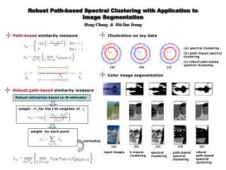
Line Drawings Training set 1 Favor connectedness Training set 2 Favor direction continuity Examples of testing segmentation trained with Training set 2 Examples of testing segmentation trained with Training set 1
Conclusions • Two sets of algorithms are presented – one for spectral clustering and one for learning the similarity matrix. • Minimization of a single cost function w.r.t. its two arguments leads to these algorithms. • The approximation scheme is efficient. • New approach is more robust to irrelevant features than current methods.