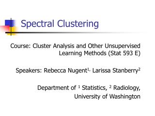
Spectral Clustering
Spectral Clustering. Course: Cluster Analysis and Other Unsupervised Learning Methods (Stat 593 E) Speakers: Rebecca Nugent 1, Larissa Stanberry 2 Department of 1 Statistics, 2 Radiology, University of Washington. Outline. What is spectral clustering?

Spectral Clustering
E N D
Presentation Transcript
Spectral Clustering Course: Cluster Analysis and Other Unsupervised Learning Methods (Stat 593 E) Speakers: Rebecca Nugent1, Larissa Stanberry2 Department of 1 Statistics, 2 Radiology, University of Washington
Outline • What is spectral clustering? • Clustering problem in graph theory • On the nature of the affinity matrix • Overview of the available spectral clustering algorithm • Iterative Algorithm: A Possible Alternative
Spectral Clustering • Algorithms that cluster points using eigenvectors of matrices derived from the data • Obtain data representation in the low-dimensional space that can be easily clustered • Variety of methods that use the eigenvectors differently
Data-driven Method 1 Method 2 matrix Data-driven Method 1 Method 2 matrix Data-driven Method 1 Method 2 matrix
Spectral Clustering • Empirically very successful • Authors disagree: • Which eigenvectors to use • How to derive clusters from these eigenvectors • Two general methods
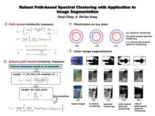
Method #1 • Partition using only one eigenvector at a time • Use procedure recursively • Example: Image Segmentation • Uses 2nd (smallest) eigenvector to define optimal cut • Recursively generates two clusters with each cut
Method #2 • Use k eigenvectors (k chosen by user) • Directly compute k-way partitioning • Experimentally has been seen to be “better”
Spectral Clustering Algorithm Ng, Jordan, and Weiss • Given a set of points S={s1,…sn} • Form the affinity matrix • Define diagonal matrix Dii=Skaik • Form the matrix • Stack the k largest eigenvectors of L to form the columns of the new matrix X: • Renormalize each of X’s rows to have unit length. Cluster rows of Y as points in R k
Cluster analysis & graph theory • Good old example : MST SLD Minimal spanning tree is the graph of minimum length connecting all data points. All the single-linkage clusters could be obtained by deleting the edges of the MST, starting from the largest one.
Cluster analysis & graph theory II • Graph Formulation • View data set as a set of vertices V={1,2,…,n} • The similarity between objects i and j is viewed as the weight of the edge connecting these vertices Aij. A is called the affinity matrix • We get a weighted undirected graph G=(V,A). • Clustering (Segmentation)is equivalent topartition of G into disjoint subsets. The latter could be achieved by simply removing connecting edges.
Nature of the Affinity Matrix “closer” vertices will get larger weight Weight as a function ofs
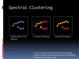
Simple Example • Consider two 2-dimensional slightly overlapping Gaussian clouds each containing 100 points.
Magics • Affinities grow as grows • How the choice of s value affects the results? • What would be the optimal choice for s?
Spectral Clustering Algorithm Ng, Jordan, and Weiss • Motivation • Given a set of points • We would like to cluster them into k subsets
Algorithm • Form the affinity matrix • Define if • Scaling parameter chosen by user • Define D a diagonal matrix whose (i,i) element is the sum of A’s row i
Algorithm • Form the matrix • Find , the k largest eigenvectors of L • These form the the columns of the new matrix X • Note: have reduced dimension from nxn to nxk
Algorithm • Form the matrix Y • Renormalize each of X’s rows to have unit length • Y • Treat each row of Y as a point in • Cluster into k clusters via K-means
Algorithm • Final Cluster Assignment • Assign point to cluster j iff row i of Y was assigned to cluster j
Why? • If we eventually use K-means, why not just apply K-means to the original data? • This method allows us to cluster non-convex regions
User’s Prerogative • Choice of k, the number of clusters • Choice of scaling factor • Realistically, search over and pick value that gives the tightest clusters • Choice of clustering method
Advantages/Disadvantages • Perona/Freeman • For block diagonal affinity matrices, the first eigenvector finds points in the “dominant”cluster; not very consistent • Shi/Malik • 2nd generalized eigenvector minimizes affinity between groups by affinity within each group; no guarantee, constraints
Advantages/Disadvantages • Scott/Longuet-Higgins • Depends largely on choice of k • Good results • Ng, Jordan, Weiss • Again depends on choice of k • Claim: effectively handles clusters whose overlap or connectedness varies across clusters
Affinity Matrix Perona/Freeman Shi/Malik Scott/Lon.Higg 1st eigenv. 2nd gen. eigenv. Q matrix Affinity Matrix Perona/Freeman Shi/Malik Scott/Lon.Higg 1st eigenv. 2nd gen. eigenv. Q matrix Affinity Matrix Perona/Freeman Shi/Malik Scott/Lon.Higg 1st eigenv. 2nd gen. eigenv. Q matrix
Inherent Weakness • At some point, a clustering method is chosen. • Each clustering method has its strengths and weaknesses • Some methods also require a priori knowledge of k.
One tempting alternative The Polarization Theorem (Brand&Huang) • Consider eigenvalue decomposition of the affinity matrix VLVT=A • Define X=L1/2VT • Let X(d) =X(1:d, :) be top d rows of X: the d principal eigenvectors scaled by the square root of the corresponding eigenvalue • Ad=X(d)TX(d) is the best rank-d approximation to A with respect to Frobenius norm (||A||F2=Saij2)
The Polarization Theorem II • Build Y(d) by normalizing the columns of X(d) to unit length • Let Qij be the angle btw xi,xj – columns ofX(d) • Claim As A is projected to successively lower ranks A(N-1), A(N-2), … , A(d), … , A(2), A(1), the sum of squared angle-cosines S(cos Qij)2 is strictly increasing
Brand-Huang algorithm • Basic strategy: two alternating projections: • Projection to low-rank • Projection to the set of zero-diagonal doubly stochastic matrices (all rows and columns sum to unity) • stochastic matrix has all rows and columns sum to unity
Brand-Huang algorithm II • While {number of EV=1}<2 do • APA(d)PA(d) … • Projection is done by suppressing the negative eigenvalues and unity eigenvalue. • The presence of two or more stochastic (unit)eigenvalues implies reducibility of the resulting P matrix. • A reducible matrix can be row and column permuted into block diagonal form
References • Alpert et al Spectral partitioning with multiple eigenvectors • Brand&Huang A unifying theorem for spectral embedding and clustering • Belkin&Niyogi Laplasian maps for dimensionality reduction and data representation • Blatt et al Data clustering using a model granular magnet • Buhmann Data clustering and learning • Fowlkes et al Spectral grouping using the Nystrom method • Meila&Shi A random walks view of spectral segmentation • Ng et al On Spectral clustering: analysis and algorithm • Shi&Malik Normalized cuts and image segmentation • Weiss et al Segmentation using eigenvectors: a unifying view