5. Quantum Theory
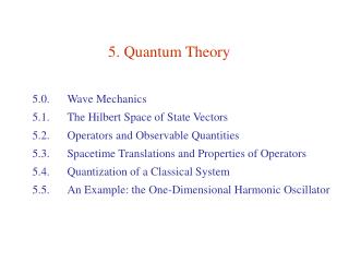
5. Quantum Theory. 5.0. Wave Mechanics 5.1. The Hilbert Space of State Vectors 5.2. Operators and Observable Quantities 5.3. Spacetime Translations and Properties of Operators 5.4. Quantization of a Classical System 5.5. An Example: the One-Dimensional Harmonic Oscillator.

5. Quantum Theory
E N D
Presentation Transcript
5. Quantum Theory 5.0. Wave Mechanics 5.1. The Hilbert Space of State Vectors 5.2. Operators and Observable Quantities 5.3. Spacetime Translations and Properties of Operators 5.4. Quantization of a Classical System 5.5. An Example: the One-Dimensional Harmonic Oscillator
5.0. Wave Mechanics • Cornerstones of quantum theory: • Particle-wave duality • Principle of uncertainty Planck’s constant History: Planck: Empirical fix for black body radiation. Einstein: Photo-electric effect → particle-like aspect of “waves”. de Broglie: Particle-wave duality. Thomson & Davisson: Diffraction of electrons by a crystal lattice. Schrodinger: Wave mechanics.
Wave mechanics State of a “particle” is represented by a (complex) wave function Ψ( x, t ). Probability of finding the particle in d 3x about x at t = P = probability density if Ψ( x, t ) is called normalized if c = 1. Pd 3x = relative probability if Ψ cannot be normalized. E.g., free particle: (1st) quantization: → r-representation:
Hamiltonian : → Time-dependent Schrodinger equation : c.f. Hamilton-Jacobi equation Time-independent Schrodinger equation :
5.1. The Hilbert Space of State Vectors Specification of a physical state: Maximal set of observables M = { A, B, C, …}. → Pure quantum state specified by values { a, b, c, … } assumed by S. Assumption: Every possible instantaneous state of a system can be represented by a ray (direction) in a Hilbert space. (see Appendix A.3) Hilbert spaces are complex linear vector spaces with possibly infinite dimensions. • φ | = 1-form dual to | φ = | φ † Inner product is sesquilinear : α, β C, → Norm / length / magnitude of | φ is
| φ is normalized if Maximal set M = { A, B, C, …} → pure states are given by | a, b, c, … . Probability of measuring values { a, b, c, … } from a state | Ψ is → orthonormality → → Completeness else
If a takes on continuous values, Example: 1-particle system with x as maximal set. orthonormality completeness Ψ (x) = wave function
5.2. Operators and Observable Quantities Operator: E.g., identity operator: Linear operators: α, β C Observables are represented by linear Hermitian operators. Let the maximal set of observables be M = { A, B, C, …}. If we choose | a,b,c,… as basis vectors, then the operators are defined as Eigen-equations eigenvalues eigenvectors …
Expectation value of A: AdjointA† of A is defined as: → A is self-adjoint / hermitian if
Consider 2 eigenstates, | a1 and | a2, of A. → If A is hermitian, Hence, → Eigenvalues of a hermitian operator are all real. → Eigenstates belonging to different eigenvalues of a hermitian operator are orthogonal.
Algebraic Operations between Operators Addition: Product: Commutator: Analytic functions of A are defined by Taylor series. Ex. 5.7 Caution: unless If B is hermitian, then → ( A is unitary )
5.3. Spacetime Translations and Properties of Operators Time Evolution: Schrodinger Picture Each vector in Hilbert space represents an instantaneous state of system. U is the time evolution operator Normalization remains unchanged : → U is unitary Setting we can write where If H is time-independent, → H = Hamiltonian c.f. Liouville eq.
Heisenberg Picture | Ψ (t) is not observable. Observable: for time independent H → A is conserved if it commutes with H. H is conserved. Classical mechanics: Possible rule: ( Not always correct ) Example: Canonical commutation relations
Alternative derivation: Classical translational generator: → All components of x or p should be simultaneously measurable → → Consider → → See Ex.5.3 for higher order terms → H independent of x (translational invariant)
Classical mechanics: Conserved quantity ~ L invariant under corresponding symmetry transformation Quantum mechanics: Conserved operator = generator of symmetry transformation Example: Angular Momentum
5.4. Quantization of a Classical System Canonical quantization scheme: Classical Quantum Schrodinger Heisenberg • Difficulties: • Generalized coordinates may not work. • Remedy: Stick with Cartesian coordinates. • Ambiguity. E.g., AB when Possible remedy: use Remedy: use pi . • Constrainted or EM systems with Reminder: velocity is ill-defined in QM.
Wave functions: x-representation (Taylor series) → Many bodies:
5.5. An Example: the One-Dimensional Harmonic Oscillator Some common choices of maximal sets of observables: { x } : coordinate (x-) representation { p } : momentum (p-) representation { E } : energy (E-) representation { n } : number (n-) representation n-representation Basis vectors are eigenstates of number operator: Lowering (annihilation) operator: Raising (creation) operator: Canonical quantization:
→ → → … → → Setting cn and bn real gives
Exercise: Show that if n is restricted to the values 0 and 1, then the commutator relation must be replaced by the anti-commutator relation
For the harmonic oscillator, if we set then → Hence, basis { | n } is also basis of the E-representation. The nth excited state contains n vibrons, each of energy ω. → →
x-representation: → where → so that with Using one can show where and
The x- and p- representations are Fourier transforms of each other. where so that Similarly where In practice, ψ (x) is easier to obtain by solving the Schrodinger eq. with appropriate B.C.s
Let V(x) → 0 as |x| → . For E < 0, ψn(x) is a bound state with discrete eigen-energies εn. For E > 0, ψk(x) is a scattering state with continuous energy spectrum ε(k). However, scattering problems are better described in terms of the S matrix, scattering cross sections, or phase-shifts.