Download

1 / 17
170 likes | 194 Vues
Integrating Reserve Risk Models into Economic Capital Models. Stuart White, Corporate Actuary Casualty Loss Reserve Seminar, Washington D.C. 18-19 September 2008. Disclaimer.

E N D
Integrating Reserve Risk Models into Economic Capital Models Stuart White, Corporate Actuary Casualty Loss Reserve Seminar, Washington D.C. 18-19 September 2008
Disclaimer • The views and opinions expressed in this presentation are solely those of the Speaker and not those of XL Capital Ltd or any of its subsidiary companies
Integrating Reserve Risk into Economic Capital Models • Selecting Reserve Risk Distributions • Evaluate model fit • Interpreting model output • Integrating Reserve Risk • Fitting distributions to held reserves • One year vs ultimate • Correlation or dependence structure
1) Selecting Reserve Risk Distributions • Consider multiple methods • Bootstrap, Mack, other • Paid vs Incurred • Historical reserve data • Industry data • Consistency with current year pricing distributions / RDS / scenario tests • How does the output compare with regulator and rating agency capital benchmarks?
Evaluate model fit • Practical methods • How well does the reserve predicted by the model match the held reserve? If no, then can you trust the predicted standard deviation as well? • Do relationships across lines make sense? • Back-testing – Compare historical prior year development to model predictions • Changes to the mix of business or terms and conditions. May need to adjust the data or bear in mind when selecting results.
Back-test reserve ranges 80% confidence interval • A back-test compares reserve development over a one-year period against the original estimate of a reserve range • In this exhibit red indicates a strengthening of reserves, green a release
Evaluate model fit • Statistical methods • “Need to check the reasonableness of model assumptions” • Plot residuals – do they match assumed distributions? • Variance or Heteroskedasticity (can be a problem across development periods or underwriting years) • Outliers • Leverage – identify points with excessive influence on model results • Significance tests of model parameters • Compare goodness of fit with historical data • On following two slides example output of good and bad fits from a standard statistical package
(Good Fit) Points are along 45 deg line Relatively flat trend in variance of residuals May want to investigate point #72, but not an extreme outlier
(Poor Fit) Points deviate from 45 deg line Variance increasing with size of predicted values
Interpreting model output • Plot the output of model iterations • Benefit of fitting a distribution to simulated model output • More stable tail values • Model Output may be closer to a “shifted” lognormal distribution • How do you measure the coefficient of variation? • Comparability across methods
Interpreting model output:Plot distributions Graphing distributions scaled to a common mean gives a good basis for comparison and sense checking results across different methods or lines of business
Interpreting model output:Shifted lognormal example • Mean of lognormal distribution is: • 30%+40% = 70% • Coefficient of variation is: • 30% / 70% = 42.9% • CV for un-shifted distribution is: • 30% / 40% = 75% • This can be a real issue when comparing distributions from different models that are of different shapes. The shift is important! • continued …
Interpreting model output:Shifted lognormal example continued • Suppose your model produced the distribution described on the previous slide • But you only measured the mean and CV (70% and 42.9%), and then applied this to a lognormal distribution • This widens a typical reserve range interval (e.g. 10-90 percentile), but reduces capital percentiles (e.g. 99 or 99.5):
2) Integrating Reserve Risk Fitting distributions to held reserves • What if modeled reserves don’t match held reserves? • Decision on whether to scale or shift output distributions in order to match model means (exactly the same issues shown in the previous example) • Incurred claims models predict the variability in IBNR. Therefore need to make an assumption about case reserves (fixed or stochastic?) • Exclusions from modeled data: • Large losses • Expense reserves, unrecoverables • Ceded amounts
One Year vs Ultimate • Does it makes sense to aggregate ultimate reserve risk distributions with different tail lengths? • Consider time horizon of other risk categories, which are often looked at over a single year • Asset • Credit • FX • Operational • How would you combine these with an ultimate reserve risk distribution? • Implication would be to use a one-year reserve distribution, which makes aggregation with other risks more straightforward
One Year vs Ultimate • Therefore either need a methodology to produce one-year reserve risk volatilities or a way to transform ultimate distributions • Run-off ultimate using loss development pattern • Wacek – “The path of the ultimate loss ratio” (CAS Forum Winter 2007) • Adjust confidence level used to derive capital • For example the FSA approach that 97.5% over a 5 year time horizon is equivalent to 99.5% over 1 year • May use the multi-year default curves published by rating agencies combined with the expected duration of capital held to estimate this
Correlation or dependence structure • Possibilities: • Large correlation/copula matrix • Multiple stages of aggregation • Dependence • An example of a multi-stage approach would be to model reserve and current year risk together within a model • A stochastic claims model (such as bootstrap) can be adjusted to produce loss projections for the current year • Model a rate level index using time series to capture inter-year dependence • Combine the two for a model that considers both current and prior year risk • Dependence structures would include: • Linking reserve or underwriting distributions to common factors. These may be items such as shock losses or economic variables such as inflation or interest rates • Such approaches offer a more detailed link with other risks such as asset and credit