Section 3-1 to 3-2, 3-5

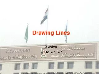
1. Drawing Lines Section 3-1 to 3-2, 3-5 Some of the material in these slides may have been adapted from university of Virginia, MIT, and ÅboAkademi University

2. Line Algorithms • Drawing 2-D lines: a case study in optimization • We will use Professor Leonard McMillan’s web-based lecture notes (then at MIT, now at UNC) • http://graphics.lcs.mit.edu/classes/6.837/F98/Lecture5 • His examples are in Java, but the correspondences are obvious.

3. Our first adventure into scan conversion. • Line drawing is our first adventure into the area of scan conversion. • The need for scan conversion, or rasterization, techniques is a direct result of scanning nature of raster displays (thus the names). • Algorithms are fundamental to both 2-D and 3-D computer graphics • Transforming the continuous into this discrete (sampling) • Line drawing was easy for vector displays • Most incremental line-drawing algorithms were first developed for pen-plotters • We will gradually evolve from the basics of algebra to the famous Bresenham line-drawing algorithms • We will look at others

4. Quest for the Ideal Line • Important line qualities: • Continuous appearance • Uniform thickness and brightness • Turn on the pixels nearest the ideal line • How fast is the line generated • Line usually specified by slope mand a y-axis intercept called b. • Generally in computer graphics, a line will be specified by two endpoints.

5. Simple Line Based on the simple slope-intercept algorithm from algebra y = m x + b public void lineSimple(int x0, int y0, int x1, int y1, Color color) { int pix = color.getRGB(); intdx = x1 - x0; intdy = y1 - y0; raster.setPixel(pix, x0, y0); if (dx != 0) { float m = (float) dy / (float) dx; float b = y0 - m*x0; dx = (x1 > x0) ? 1 : -1; while (x0 != x1) { x0 += dx; y0 = Math.round(m*x0 + b); raster.setPixel(pix, x0, y0); } } }

6. Does this algorithm work? This algorithm works well when the desired line's slope is less than 1, but the lines become more and more discontinuous as the slope increases beyond one. Since this algorithm iterates over values of x between x0 and x1 there is a pixel drawn in each column. When the slope is greater than one then often more than one pixel must be drawn in each column for the line to appear continuous. LineSimple Applet

7. Improved Line Drawing Algorithm Problem:lineSimple does not give satisfactory results for slopes > 1. Solution: symmetry: The assigning of one coordinate axis the name x and the other y was an arbitrary choice. Notice that line slopes of greater than one under one assignment result in slopes less than one when the names are reversed.

8. lineImproved(int x0, int y0, int x1, int y1) { int dx = x1 - x0; int dy = y1 - y0; raster.setPixel(pixel1, x0, y0); if (Math.abs(dx) > Math.abs(dy)) { // slope < 1 // compute slope: float m = (float) dy / (float) dx; float b = y0 - m*x0; dx = (dx < 0) ? -1 : 1; while (x0 != x1) { x0 += dx; raster.setPixel(pix, x0, Math.round(m*x0 + b)); } } else if (dy != 0) { // slope >= 1 // compute slope: float m = (float) dx / (float) dy; float b = x0 - m*y0; dy = (dy < 0) ? -1 : 1; while (y0 != y1) { y0 += dy; raster.setPixel(pixel1, Math.round(m*y0 + b), y0); } } }

9. Algorithm Comment Notice that the slope-intercept equation of the line is executed at each step of the inner loop. Line Improved Applet

10. Line Drawing Optimization – Optimize Inner Loop Optimize those code fragments where the algorithm spends most of its time Often these fragments are inside loops. Remove unnecessary method invocations: Replace Math.round(m*x0 + b) with (int)(m*y0 + b + 0.5). Use incremental calculations: Consider the expression : y = (int)(m*x + b + 0.5) The value of y is known at x0 (i.e. it is y0 + 0.5) Future values of y can be expressed in terms of previous values with a difference equation: yi+1 = yi + m; or yi+1 = yi - m; Adding all these modifications to the lineModified() method, we obtain a new  line drawing method called a Digital Differential Analyzer or DDA for short.

11. Low level Optimization Low-level optimizations are dubious, because they depend on specific machine details. However, a set of general rules that are more-or-less consistent across machines include: Addition and Subtraction are generally faster than Multiplication. Multiplication is generally faster than Division. Using tables to evaluate discrete functions is faster than computing them Integer calculations are faster than floating-point calculations. Avoid unnecessary computation by testing for various special cases. The intrinsic tests available to most machines are greater than, less than, greater than or equal, and less than or equal to zero (not an arbitrary value).

12. Applications of Low-level Optimizations Notice that the slope is always rational (a ratio of two integers). m = (y1 - y0) / (x1 - x0) Also notice that the incremental part of the algorithm never generates a new y that is more than one unit away from the old one (because the slope is always less than one) yi+1 = yi + m Thus, if we maintained the only fractional part of y we could still draw a line by noting when this fraction exceeded one. If we initialize fraction with 0.5, then we will also handle the rounding correctly as in our DDA routine: fraction += m; if (fraction >= 1) { y = y + 1; fraction -= 1; }

13. Bresenham's line drawing algorithm y is now an integer. Can we represent the fraction as an integer? After we draw the first pixel (which happens outside our main loop) the correct fraction is: fraction = 1/2 + dy/dx If we scale the fraction by 2*dx the following expression results: scaledFraction = dx + 2*dy So the incremental update becomes: scaledFraction += 2*dy // 2*dx*(dy/dx) & our test must be modified to reflect the new scaling: if (fraction >= 1) { y = y + 1; fraction -= 1; }  if (scaledFraction >= 2*dx)

14. Bresenham's line drawing algorithm This test can be made against a value of zero if the inital value of scaledFraction has 2*dx subtracted from it. Giving, outside the loop: OffsetScaledFraction = dx + 2*dy - 2*dx = 2*dy - dx So the inner loop becomes         OffsetScaledFraction += 2*dy        if (OffsetScaledFraction >= 0)         {            y = y + 1;            fraction -= 2*dx;        } We might as well double the values of dy and dx (this can be accomplished with either an add or a shift outside the loop). The resulting method is known as Bresenham's line drawing algorithm Bresenham's Line Drawing Applet

15. Bresenham's Line-Drawing Algorithm for |m| < 1 Drawing a line from (x0,y0) to (x1,y1) assumingx1>x0 Input the two line endpoints and store the left endpoint in (x0,y0) Load (x0,y0) into the frame buffer; that is, plot the first point. Calculate constants dx, dy=abs(y1-y0), 2dy, and 2dy–2dx, ystep (=1 for y1>y0 or = -1 for y1<y0) and obtain the starting value for the decision parameter as P0= 2dy – dx At each xkalong the line, starting at k = 0, perform the following test: If Pk< 0, the next point to plot is (xk+ 1, yk) and Pk+1=Pk+2dy Otherwise, the next point to plot is (xk+1 , yk+ystep) and Pk+1= Pk+ 2dy – 2dx Repeat step 4 dx times.