Importance of ozone Overview the ARPEGE-Climat ozone parameterization

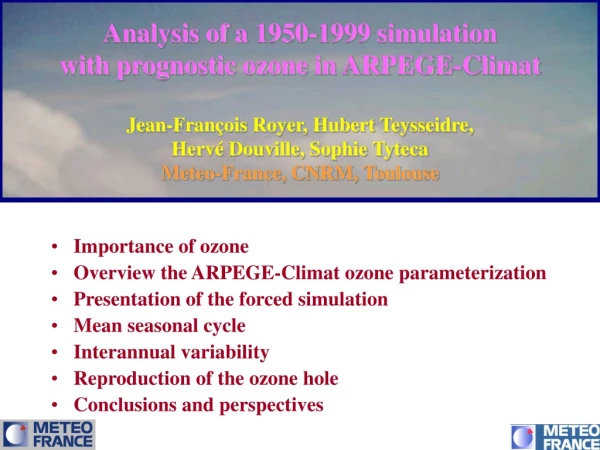
1. Analysis of a 1950-1999 simulation with prognostic ozone in ARPEGE-ClimatJean-François Royer, Hubert Teysseidre, Hervé Douville, Sophie TytecaMeteo-France, CNRM, Toulouse • Importance of ozone • Overview the ARPEGE-Climat ozone parameterization • Presentation of the forced simulation • Mean seasonal cycle • Interannual variability • Reproduction of the ozone hole • Conclusions and perspectives

2. Importance of ozone • Absorption of UV and IR radiation • Complex tropospheric and stratospheric chemistry • Long term trends observed in total ozone • Stratospheric ozone depletion over the South Pole (ozone hole) since the 1970s • Many studies have shown evidence of the impact of anthropic perturbations on atmospheric chemistry (CFCs, NOx, CH4, CO …) • Stratospheric trends due to the inverse greenhouse effect • Impact of stratospheric cooling on ozone photochemistry and ozone catalytic destruction by chlorine compounds • WMO/UNEP Scientific Assessment of Ozone Depletion (1998, 2002)

3. Purpose of the presentation • To document the capacity the ARPEGE-Climat GCM, that includes a ozone as a prognostic variable with a simple parameterization of its photochemistry, to reproduce the main characteristics of ozone distribution • To evaluate its capacity at simulating its observed long term evolution in response to SST, greenhouse gas forcing, and changing composition of the atmosphere • To identify the impact and signature of anthropic perturbations on the evolution of the ozone layer

4. Description of the simulations • ARPEGE-Climat version 3 • Dynamics and resolution: • Semi-lagrangian version with ozone transport • T63 linear grid (128x64 points) • 45 levels in the vertical • Physical parameterizations • State-of-the-art GCM physics (convective and large-scale precipitation, interactive clouds, turbulence, land surface processes ISBA) • ECMWF (Fouquart, Morcrette) radiation scheme (every 3 hours) with major greenhouse gases (CO2, CH4, N20, O3, CFC-11 and CFC-12) • Sulfate Aerosols: direct and indirect effects (Boucher and Lohman parameterization implemented by Hu RM et al 2002) • prognostic computation of ozone concentration

5. The forced simulation • 50 year simulation starting in 1950 • Observed GHGs: • CO2 • CH4 • N2O • CFC11 • CFC12+(others) • Aerosols concentrations (J Penner) • The sea surface temperatures (SSTs) are specified according to the observed monthly means (Reynolds analyses) over the period 1960-2000 • Ozone transport and simplified photochemistry • Derived from the 2D zonal model MOBIDIC • (MOdel of BI-DImensional Chemistry)

6. MOBIDIC Stratospheric chemistry Zonal-mean coefficients for O3 parameterization CO2 CH4 N2O CFCs Cl Zonal Averages (10 years) ARPEGE-Climat AGCM Aerosols Climate statistics ISBA Land surface Sea-ice Observed SSTs (monthly-mean)

7. The 2D photochemical model MOBIDIC [Cariolle, CNRM, 1984 ; Teyssèdre, UPS, 1994] • 2 dimensions (latitude, pressure) • thermodynamical forcings from ARPEGE-Climat (T, v*, w*, Kyy, Kyz, Kzz) • stratospheric chemistry : 56 species, 175 reactions • studies of atmospheric impact (supersonic aircraft) • for ozone linear parametrisation : • chemical equilibrium => (P-L) ; rO3 ; T ;  • +/- 10% perturbation => new equilibrium :  (P-L) /  rO3 ;  (P-L) /  T ;  (P-L) /  

8. linearised ozone chemistry [Cariolle and Déqué, JGR, 1986]  rO3/  t = (P-L) + (rO3 - rO3)  (P-L) /  rO3 +(T – T)  (P-L) /  T +( – )  (P-L) /   - Khet (Cly(year))2rO3 from 3D GCM from 2D photochemical model ( , p) (P-L) : ozone production-loss term rO3 : ozone mixing ratio T : temperature  : ozone column above gridpoint Khet : heterogeneous chemistry Cly(year) : total chlorine for given year

9. (P-L)

10. rO3  (P-L) /  rO3

11. T  (P-L) /  T

12.   (P-L) /  

13. Khet (T  195 K under sunlight conditions)

14. Validation of the resultsComparison of the climate of the 60s and 90s • Maps of the differences between 20-year mean simulated distributions for two different periods • 1950-1969 • 1980-1999 • Total ozone column (DU= Dobson Units ~ mm O3 at STP) • Ozone concentration (volume mixing ratio in ppmv) • Validation of the ozone distribution • Comparison with UGAMP 5-year ozone climatology 1985-1989 • Monthly, 2.5° x 2.5°, 47 levels • (Li and Shine, 1995) • Available at BADC

15. Ozone column (DU) 1985-1989 UGAMP ARPEGE-Climat March 300 400 Septembre

16. 20-year mean 1980-1999: isolines Difference from 1950-1969 mean: colour scale ARPEGE-Climat March

17. Ozone over NH

18. 20-year mean 1980-1999: isolines Difference from 1950-1969 mean: colour scale ARPEGE-Climat September

19. SP September

20. Seasonal evolution of the O3 column (DU) UGAMP ARPEGE-Climat

21. Ozone 20-year mean 1980-1999: isolines Difference from 1950-1969 mean: colour scale

22. Vertical distribution of O3 concentration (ppmv) 1985-1989 UGAMP ARPEGE-Climat Annual mean

28. Seasonal evolution at 10 hPa

29. Montly anomalies with respect to 1950-1969 global average Montly anomalies with respect to 1950-1969 global average 10 hPa ozone 10 hPa temperature 1999 1950 1950 1999 surface Ozone column surface temperature 1999 1999 1950 1950

30. Monthly anomaly with respect to 1950-1969 averagefor ozone column (DU) over South Pole (80-90°S)

34. Conclusions • The ozone transport and simple parameterization of its sources and sinks is able to reproduce the geographical and seasonal distribution patterns of total ozone column • The vertical distribution of ozone in the stratosphere is simulated realistically • In response to the increase of CFCs the model simulates a reduction of ozone in the upper stratosphere due to its increased destruction by released chlorine • This leads to a cooling in the upper stratosphere due to the reduction of UV absorption • However due to the tropospheric response the total ozone column increases slightly, which is not in agreement with observations

35. Conclusions (2) • The heterogeneous chemistry parameterization is able to reproduce the destruction of ozone by PSCs in the South Polar vortex at the begining of Austral spring • Though the structure of the simulated ozone hole is realistic its intensity is too weak • Need to revise and adjust the destruction coefficient for heterogeneous chemistry to improve the efficiency of the parameterization in future C20C simulations