Download
1 / 41
410 likes | 449 Vues
This lecture provides an overview of the basic principles of cosmology, including the homogeneity and isotropy of the universe, the expansion of space, the Big Bang theory, and the formation of structure. It also explores the historical milestones of cosmology and the methods used to measure distances in the universe.

E N D
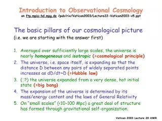
Introduction to Observational Cosmologyon ftp.mpia-hd.mpg.de/pub/rix/Vatican2003/Lecture22-Vatican2003-v5.ppt The basic pillars of our cosmological picture (i.e. we are starting with the answer first) • Averaged over sufficiently large scales, the universe is nearly homogeneous and isotropic (=cosmological principle) • The universe, i.e. space itself, is expanding so that the distance D between any pairs of widely separated points increases as dD/dt~D (=Hubble law) • (?) the universe expanded from a very dense, hot initial state(=big bang) • The expansion of the universe is determined by its mass/energy content and the laws of General Relativity • On “small scales” (<10-100 Mpc) a great deal of structure has formed through gravitational self-organization. Vatican 2003 Lecture 20 HWR
Historical Milestones of Cosmology • 1920s :Galaxies (=“nebulae”) are distinct entities of stars like our Milky Way Universe // Milky Way Note: Nearly co-identical with Einstein's General Relativity (1916) Distances in the Universe First measure of characteristic distance to other galaxies: Öpik (1922) measured the rotation speed of the Andromeda galaxy and determined the distance at which its mass to light ratio equals the Milky Way's: (M/L)And (M/L)* in MW withand DAnd 0.5 Mpc Hubble (1929) measured distances to galaxies using Cepheids (M31, M33) and brightest stars, obtaining similar distances. Vatican 2003 Lecture 20 HWR
Expansion of the Universe • 1929 and 1931 Hubble (and Humason) • Fainter (and hence more distant) galaxies recede from the Milky Way at a rate proportionate to their (estimated) distance. • Big problem: what is the proportionality constant, the distance scale? (Hubble got it wrong by a factor of 8) 10,000 km/s 1000 km/s Mean apparent magnitude Vatican 2003 Lecture 20 HWR
Redshift • Observational result: The measured redshift (often falsely interpreted as "recession velocity") of an object(0 = rest wavelength) is proportional to the (independently) measured distance D of an object (but with some scatter!!) • Longstanding problem:We need the absolute distance measure to get the slope of the relation v = H0 · D ; the proportionality constant is called "Hubble constant". More appropriate qualitative interpretation: The universe/space has expanded by a factor of (1+z) between emission and observation of the light. Vatican 2003 Lecture 20 HWR
Quasars • In 1963 Maarten Schmidt (+Jesse Greenstein) found that a radio source was actually a galaxy nucleus at z @ 0.16 that was by far the most distant object at the time • 1965 Quasars with redshifts z>2 found! cosmological look-back! Vatican 2003 Lecture 20 HWR
Cosmic Microwave Background (CMB) • “Afterglow” of the big-bang • Discovered by Penzias and Wilson (1965) • glimpse of the universe in its infancy <T> = 2.73°K Small temperature fluctuations arising from early weak fluctuations in the matter distribution Vatican 2003 Lecture 20 HWR
Distance Measurements • Measuring distances is one of the most fundamental tasks of astronomy, needed to: • Convert angular sizes to physical sizes • Convert apparent flux to absolute luminosity • Determine relative geometry of different ojects • Determine look-back time • Measuring astronomical distances is difficult, there are three types of methods: • Geometric methods • Standard Candles • Direct physical estimates (gravitational lensing, CMB) Vatican 2003 Lecture 20 HWR
Reid 1997 Geometric Distance Measurements • Parallax measurements i.e. Earth’s motion reflex • State of the art: Hipparchos (ESA Mission in the 1990s) Parallax accuracy of 0.9 milli-arcseconds distances to 1 kpc Application Calibrate nearby (~ 100pc) stars of the appropriate metallicity match to globular cluster main-sequence Distance to globular clusters (to 5%), which contain cepheids Vatican 2003 Lecture 20 HWR
Standard Candles Approach: • Select objects whose intrinsic luminosity can be estimated, either from physical first principles, from empirical calibrations of nearby examples or can be inferred from another distance-independent observable. • Instrinsic luminosity + apparent flux distance (modulus) Examples: • Cepheids: luminosity estimate from their pulsation period • Spiral Galaxies: luminosity estimate from their disk rotation curve • Type-Ia Supernovae (SNIa): luminosity estimate from their light-curve shape Vatican 2003 Lecture 20 HWR
lightcurves Cepheid Distances • E.g. HST Key-Project to measure Hubble constant, H0 (Freedman, Kennicutt,Mould, et al.) • Compare Cepheid brightness in M81 to LMC and local Milky Way Cepheids DM81=3.63+-0.34 • This way we can measure distances to Galaxies with where Supernovae exploded. Note:for nearby (<50Mpc) galaxies distance and redshift are correlated with considerable scatter Measuring H0 is not easy Vatican 2003 Lecture 20 HWR
Perlmutter etal 2002 Supernova Type Ia Distances • SN Ia: white dwarf stars near the Chandrasekhar mass limit (1.4 Msun), where Carbon and Oxygen burn explosively. • Most luminous variety of Supernova. Can be seen to z>1! Vatican 2003 Lecture 20 HWR
SN Ia as Pseudo-Standard Candles Phillips, Hamuy, Ries, Kirshner and others ~1996 • Intrinsically bright SN Ia decline slower • SN Ia: H0=67+-5 km/s/Mpc (Current estimate (all methods): H0=70+-3) Note: • still needs Cepheid calibration • Galaxy velocities differ from the local mean by ~300 km/s systematic uncertainty in H0 with correction Vatican 2003 Lecture 20 HWR
Distant Supernovae • The distance modulus M-m to a certain redshift z depends on the expansion history, not just the current expansion rate. • Type-Ia Supernovae can be seen to great distances: z>1 probes of the expansion history. • 1998: expansion of the Universe is accelerating (!?) • Riess etal 1998, AJ, 116, 1009 • Perlmutter et al. 1999, ApJ, 517, 565 Vatican 2003 Lecture 20 HWR
Surveying Galaxies Goal: • We want to draw up a comprehensive picture of the galaxy population in either the nearby, present-day universe, or in the distant, earlier universe. • Such a “picture” includes: • the frequency of galaxies as a function of their • Luminosity • Structure (Size, bulge-to-disc ratio, etc..) • Dynamical mass • Star formation rate • Color (or spectral energy distribution) of the stellar population • the correlation of these parameters with each other. • Tully-Fisher relation, fundamental plane, star formation – color • The connection of individual galaxy properties with their “environment” (e.g. cluster or field, etc..) Ideally:we would like to know “everything” about all galaxies in a given, large volume ……… Vatican 2003 Lecture 20 HWR
Observables in Galaxy (or Star) Surveys Observables in large surveys: • Flux in a given aperture for several bands (e.g. IR, optical X-ray) • Spectra (for Dl/<l> ~0.5) and redshift (Distance +- 4Mpc) • Some morphology/structure information. Observational constraints in galaxy/cosmology surveys • For compact or unresolved objects surveys are flux-limited (separate flux limit in each observational band). • For extended objects surveys are surface brightness limited(i.e. limited by the contrast to the background) • For imaging surveys, the observed bands correspond to different rest-frame wavelengths. • As galaxies have different intrinsic spectral energy distributions, some objects will be above the survey limit in one band, but not the other. How to deal with these difficulties? Vatican 2003 Lecture 20 HWR
Some Consequences • Impracticability of nearby, volume limited samples: • Given a flux limit flim,l any object of luminosity Ll, can be seen only within an volume V=dW*(L/(4pflim,l))3/2 • In practice, it means one only needs to know the maximum volume within which the object would have in the survey From the 2DFRS Vatican 2003 Lecture 20 HWR
K-Corrections Vatican 2003 Lecture 20 HWR
Galaxy Surveys: the present-day luminosity function • Luminosity function: • basic, long-standing statistic to describe the galaxy population: described the space density of galaxies at a given luminosity (or absolute magnitude): • Often parameterized as a “Schechter function” (1976), to be a power-law at the faint end and an exponential at the brightest end, with a characteristic luminosity L* Vatican 2003 Lecture 20 HWR
The LF from SDSS (+2MASS and 2DFRS) Sloan Digital Sky Survey: Five-color digital map of the Northern sky (8000 sq. deg) with • photometry on >10,000,000 galaxies spectra (redshifts) for nearly 1,000,000 galaxies. Vatican 2003 Lecture 20 HWR
How the Sloan Digital Sky Survey (SDSS) works Vatican 2003 Lecture 20 HWR
www.sdss.org Vatican 2003 Lecture 20 HWR
bright SDSS Luminosity Function (5% of Data)Blanton et al 2001 • about 1 L* galaxy / 100 Mpc3 ; M* (now)=-20.8 in r-band (Note:by convention H0=100) • Schechter function is a good representation • LF (= abundance distribution) depends on the intrinsic color of the galaxy Vatican 2003 Lecture 20 HWR
Early type == concentrated light The Galaxy Mass (in Stars) Function • Bell et al. 2003: use galaxy colors to estimate (M/L)stars and hence Mstars Vatican 2003 Lecture 20 HWR
Compare this to the local group Vatican 2003 Lecture 20 HWR
The local size distribution of galaxies • Shen et al 2003 from SDSS Note:Size Specific Angular Momentum Vatican 2003 Lecture 20 HWR
Present-day color distribution of galaxies(Strateva etal 2001, Hogg etal 2002) Vatican 2003 Lecture 20 HWR
The Population of Galaxies at Earlier Epochs • Basic look-back approach to galaxy evolution: • Select earlier epoch (=redshift slice) and identify galaxies. • Measure their properties and compare to “now” • Milestones of such surveys: • Canada-French-Redshift Survey (CFRS): Lilly, LeFevre etal. 1990’s • LDSS and Auto-Fib Survey: Ellis, Broadhurst et al 1990’s • Hubble Deep Field: Williams et al., Madau etal. • Basic Data: • Redshifts, luminosities, SFRs(?),SEDs Vatican 2003 Lecture 20 HWR
COMBO-17 in practice 30´x30´ Vatican 2003 Lecture 20 HWR
COMBO-17 Technique Eff. [%] Wavelength [nm] Wolf, etal. 2001, A&A, 681; Wolf, Meisenheimer, Roeser, 2001, A&A, 660 Vatican 2003 Lecture 20 HWR
Fit SED and zsimultaneouslyWolf et al 2001dz~0.015works well to z~1 Vatican 2003 Lecture 20 HWR
Redshift Histograms in COMBO-17 Fields >25,000 redshifts (Wolf et al. 2002) Fields: 30´x30´each Existing comparable surveys: CFRS,CNOC2,Keck <1000 redshifts (Wm/WL)=(0.3/0.7) Incl. GOODS ! Vatican 2003 Lecture 20 HWR
Recent Evolution of the Galaxy Populationusing “COMBO-17” as an example • Sample: 30,000 galaxies to mr~24 and to z~1.2 • How did the luminosity function of galaxies evolve over the last 8x10⁹ years? • This depends very much on their SED-type (~color), assumed to be non-evolving!! • Red galaxies used to be much more rare! - Luminous, blue galaxies used to be much more common Vatican 2003 Lecture 20 HWR
Starbursts Sbc-S.B. Sa-Sbc E-Sa Global averagesWhat Light from what type of galaxies? Vatican 2003 Lecture 20 HWR
COMBO-17: How did galaxy colors change since z~1 (Bell etal 2003) . Vatican 2003 Lecture 20 HWR
The (Red)Color-Magnitude Relation • The CMR zero-point evolution is consistent with passive aging of ancient stellar populations. • But: the total mass in star in the “red-and-dead” is now twice as high as it was at z~1. Vatican 2003 Lecture 20 HWR
GEMS: Key to “internal structure”(Galaxy Evolution fromMorphology and SEDs) • Large HST program: 125+50 orbits PI: H.-W. Rix to image “extended-Chandra-Deep-Field-South” • 10,000 redshifts from COMBO-17 • 9x9 ACS tiles 150 x HDF • V and z • Limit: mz~27.5 Vatican 2003 Lecture 20 HWR
GEMS 58 1.5% of total Vatican 2003 Lecture 20 HWR
COMBO-17 (~0.7”)vs. HST/ACS Vatican 2003 Lecture 20 HWR
GEMS: Color vs Morphology • What kinds of galaxies do we select? Bulge-Dominated Disk-Dominated Interacting/Peculiar Irregulars/Clumpy . Vatican 2003 Lecture 20 HWR
Summary • Hubble constant (=distance scale) now known to 5-10% • Expansion history can now be mapped with SN Ia to z>1. • New generation of surveys (e.g. SDSS) now can present the properties of the present day galaxy population as a function of e.g. luminosity, size, color, (environment), etc.. • Properties of the galaxy population can now be mapped (samples of >10,000) to z~1 and beyond: • disappearance of luminous blue galaxies • Red galaxies are becoming redder, etc.. Vatican 2003 Lecture 20 HWR