Pixel-level Image Fusion Algorithms for Multi-camera Imaging System
380 likes | 521 Vues
Explore cutting-edge pixel-level image fusion techniques for multi-camera systems, enhancing data integration and visualization in various applications like robotics and medical imaging.

Pixel-level Image Fusion Algorithms for Multi-camera Imaging System
E N D
Presentation Transcript
Pixel-level Image Fusion Algorithms for Multi-camera Imaging System July15, 2010 Sicong Zheng Imaging, Robotics, and Intelligent Systems Lab University of Tennessee
Outline • Introduction • Literature Review • Image fusion applications • Morphing techniques • Technical Approach: Pixel-level Image Fusion Algorithm • Segmentation-based Image Fusion Approach • Weighted Average Fusion • Segment Weighted Average Fusion • Image morphing • Image Fusion Experiment Result • Graphic User Interface • Test image fusion using elementary image • Test of image fusion algorithm using multi-sensor data integration • Performance Evaluation • Performance evaluation of image fusion using Mutual information methods • Conclusions and Future Work
Introduction • Image fusion is one of the image processing technology that combining information from two or more images into a single composite image • more informative and more suitable for computer processing and human visual perception. • It is a branch of data fusion where data is displayed as arrays of numbers representing intensity, color, temperature, distance, and other scene properties. • Image fusion has been a hot topic in many related research areas such ascomputer vision, automatic object detection, remote sensing, image processing, robotics, medical imaging etc. • Multi-sensor image fusion is the process of combining relevant useful information for several images into one image.
Application of Image Fusion • Various potential applications of image fusion include image classification, aerial and satellite imaging, concealed weapon detection, robot vision, digital camera application, medical imaging etc. Applications in these areas all benefited from image fusion. Figure : The motivating applications illustrated in this figure are image recognition and classification, aerial and satellite imaging, concealed weapon detection, and robot vision (Original images courtesy of www.flir.com/thermography/americas/us, www.coli.uni-saarland.de/groups/MC/lab.html, http://www.imagefusion.org/)
Depends on different fields of applications, we have different objectives, that is why we use image fusion techniques : 1. Reduce noise, in another word, to improve Signal-to-Noise-Ratio (SNR) by averaging over several images. 2. Improve spatial resolution (super resolution) fusion of one high resolution image with others; 3. Extend the spatial domain, such as mosaic algorithm; 4. Visualize high dimensional images (multi- and hyper- spectral) as false-color images; 5. Improve image modality from multiple sensors, generate fusion results from different physical principles such as range image, thermal image, sonar image, and X-ray image. Image Fusion Objective
Multi-sensor Image Fusion • Multi-sensor image fusion provide a way to combine different types of image information effectively and could impact on the information extraction afterward • Below is a Scheme of a general multi-sensor image fusion procedure. Thesis Contribution Parameter selection Pre-processing Sensor Image Registration Post-processing Fusion Image Enhance Sensor Image Registration Sensor • Image Registration Performance Evaluation Generate Fusion Result Displayed in GUI Analysis Figure : Block Scheme of a general multi-sensor image fusion procedure. (Original image is from the image database of the Imaging, Robotics and Intelligent Systems (IRIS) Laboratory at the University of Tennessee, Knoxville)
Outline • Introduction • Literature Review • Image fusion applications • Morphing techniques • Technical Approach: Pixel-level Image Fusion Algorithm • Segmentation-based Image Fusion Approach • Weighted Average Fusion • Segment Weighted Average Fusion • Image morphing • Image Fusion Experiment Result • Graphic User Interface • Test image fusion using elementary image • Test of image fusion algorithm using multi-sensor data integration • Performance Evaluation • Performance evaluation of image fusion using Mutual information methods • Conclusions and Future Work
Image Fusion Domain Single Image Process N Image Sequence Pixel-level Fusion Fusion Result Feature Extraction Feature-level Fusion Classification Decision-level Fusion Literature Review: Image Fusion Algorithm Figure : Image fusion block scheme of different abstraction levels, pixel-level fusion, feature level fusion, decision level fusion. The level classification of various popular image fusion methods based on computation source. The feature level fusion is generated from feature-extraction for each single image. Decision level fusion is processed based on the classification from feature extraction.
Image Fusion Pixel-level image fusion Feature-level image fusion Decision-level image fusion Averaging Neural Networks Fusion Based on Fuzzy and Unsupervised FCM Brovey Region-Based Segmentation Fusion Based on Support Vector Machine PCA K-means Clustering Fusion Based on Information Level in the Regions of Images Wavelet Transform Similarity Matching to Content-Based Image Retrieval Intensity Hue Saturation (IHS) Transform Literature Review: Image Fusion Algorithm Figure : The level classification of various popular image fusion methods based on computation source. The bottom branches show the typical image fusion algorithms that fall into each fusion level. Pixel-level method works either in the spatial domain or in the transform domain. Feature-level algorithms typically segment the image into contiguous regions and fuse the regions using their properties. Decision-level fusion algorithms combine image description to fuse.
Outline • Introduction • Literature Review • Image fusion applications • Morphing techniques • Technical Approach: Pixel-level Image Fusion Algorithm • Segmentation-based Image Fusion Approach • Weighted Average Fusion • Segment Weighted Average Fusion • Image morphing • Image Fusion Experiment Result • Graphic User Interface • Test image fusion using elementary image • Test of image fusion algorithm using multi-sensor data integration • Performance Evaluation • Performance evaluation of image fusion using Mutual information methods • Conclusions and Future Work
Pixel-based Image Fusion : Segment Fusion (SF) We assume that the , , ,… , denote the N images with height ( ) and width ( ) capturing the same scene are loaded for image fusion, and the represent the output image. • Where ,The ( i=1,2,…n) represent the horizontal slice width for each of the n source images, and are the parameters defined by the end user beforehand. We use integer in our implementation. The segmentation-and-combination step always stretch the image in horizontal direction because of there are always multiple source images. The distortion result from stretch is undesirable in most applications.
Pixel-based Image Fusion : Segment Fusion (SF) Source Image 1 Source Image 2 Source Image 3 Output Image Figure : Segmentation based Image Fusion Process: 1. Segment and combine step. The three 3x3 pixel grid represent the input source images. Each image is segmented into slices and combined together in order with each width controlled by parameter. The pixel with different intensity represent corresponding source image where the pixel comes from. The result from this step is stretched along the horizontal direction.
Pixel-based Image Fusion : Segment Fusion (SF) • Linear interpolation is a first degree method that passes a straight line through every two consecutive pixels. For each pixel in the interval, the value of can be derived geometrically from the straight line between the point and. • If , i = 1, 2, 3….m is integer value. • the advantage of this linear interpolation process is that, the output image produce smoother interpolant at moderate cost. It will not be distorted in aspect ratio and is not computationally expensive. The disadvantage is that the method is not very precise and the interpolant is not differentiable at the point (m, n). Thus for even better performance, more complicated algorithms are need. In the end, the image size will grow from to . • Appropriate value k should be defined to avoid taking excessive computer memory.
Source Image Size Extension Pixel Based Interpolation Pixel-based Image Fusion : Segment Fusion (SF) Figure : Segmentation-based Image Fusion Process: 2. Interpolation Step. This step is processed along the vertical direction. Interpolation is pixel-wise based on pixels above and below. Interpolation step is used to keep the output image in the same ratio aspect.
Segment Weighted Average Fusion (SWAF) The SWAF using n parameter to control the fusion in terms of pixel aspect, and using to control the fusion in terms of intensity aspect. Assume there are N images with height ( ) and width ( ) . For this case of N source image, the same method can be used. Assuming is the weight for part of the slice image. For , N = 1, 2, 3…, where
Segment Weighted Average Fusion (SWAF) For the case of 3 source image , The SWAF using 3 parameter to control the fusion in terms of pixel aspect, and using to control the fusion in terms of intensity aspect. Whereas the coefficients are linked by the dependency relationship: For , N = 1, 2, 3…, where
Image Morphing: Image warping In general, morphing algorithms consist of two process: warping and combination or cross fading, Let us consider a transition consist of N frames in length between source image and destination image, assume we applied morphing to the source image , and eventually generate the destination image .Thus, the intensity of a pixel at (x, y) in frame n is indicated as
Image Morphing: feature based image warping Feature based image warping is used with a higher level of control over the process. The corresponding feature lines in the source and destination are predefined for morphing process. After that, this approach used lines to correlate features in the source image to features in the destination image. The relation is based on the surrounding weight, which is the fields of influence surrounding the feature lines selected.
Image Morphing: feature based image warping Where X is the pixel co-ordinate in the destination image and X’ is the corresponding pixel co-ordinate in the source image, PQ is a line segment in the destination image and P’Q’ is the corresponding line segment in the source image, Perpendicular () returns the vector perpendicular to the input vector. Where length is the length of a line, dist is the distance from the pixel to the line, and a, b, and p are constants that can be used to change the relative effect of the lines.
Outline • Introduction • Literature Review • Image fusion applications • Morphing techniques • Technical Approach: Pixel-level Image Fusion Algorithm • Segmentation-based Image Fusion Approach • Weighted Average Fusion • Segment Weighted Average Fusion • Image morphing • Image Fusion Experiment Result • Graphic User Interface • Test image fusion using elementary image • Test of image fusion algorithm using multi-sensor data integration • Performance Evaluation • Performance evaluation of image fusion using Mutual information methods • Conclusions and Future Work
Test Result for Segmented Fusion (SF) = 2, = 1, = 3 for Red A, Green B, Blue C respectively, Size 6k x 6k Source Image 1 Zoom in View of Test Image, 32x32 Source Image 2 Source Image 3 Grayscale Value of the Zoom in View 32x32
Test Result for Segmented Fusion (SF) 1. CCD Camera Image Figure4.6 Test Human Face Image Fusion from CCD Camera and Range Sensor. (Original image is from the image database of the Imaging, Robotics and Intelligent Systems (IRIS) Laboratory at the University of Tennessee, Knoxville) (a) Face Image from CCD Camera, (b) Face Image from Range Sensor, (c) Segmented Fused Image from CCD Camera Image and Range Sensor Image, 2. Range Sensor Image
Test Result for Multi-sensor image fusion based on LMS-Z210 system b. Reflectance image of Ayer buiding c. True color image of Ayer building a. Range image of Ayer building d. Preprocessed of (c) using histogram equalization . SF result, SF result Figure Pseudo colored range image of Ayer building IRIS Lab, University of Tennessee, Knoxville, from
Test Result for Segment Weighted Average Fusion (SWAF) =1, = 3, =2, = 0.37, = 0.34 For Red A, Green B, Blue C respectively 6k x 6k Zoom in View of Test Image, 256x256 Gray Intensity Value of the Zoom in View 256x256
Test Result for Segment Weighted Average Fusion (SWAF) 1. Pseudo colored range image of Franklin Greenwich 2. Reflectance image of Franklin Greenwich processed by histogram equalization 3. True color image of Franklin Greenwich processed by histogram equalization SWAF , alpha = 0.33, beta =0.33 SWAF , alpha = 0.40, beta =0.21 SWAF , alpha = 0.40, beta =0.21
Graphic User Interface Figure Screenshot of the Pixel-Based Image Fusion Graphic User Interface. The Left layout is used for basic image fusion function, and the right layout is used for visual evaluation.
FantaMorph Overview FantaMorph Features Morph 2 to unlimited images Preview and Play in real time Export morph animation to Image Sequence, AVI, Flash, Animated GIF, EXE, Screen Saver, etc. FantaMorph uses a rendering engine which makes use of OpenGL hardware acceleration. OpenGL is an industrial graphics standard and is supported by most modern video cards. updating your video card is recommended. Figure Layout of Abrosoft Fanta Morph image morphing software. The upper left window and upper right window are for source image and destination image respectively, and the lower window is for image morphing preview. The green dot on the upper window shows the position of control point. When user point cursor on the green dot of one image, the corresponding control point of the other will be highlighted automatically.
Morph Test Result Figure Examples of image morphing for geometry using feature-based image morphing algorithm
Morph Test Result Figure Deployment for large-scale urban mapping using feature-based image morphing algorithm Images of downtown Knoxville, morphing with 83 control points
Segment Fusion (SF) Computation Test In order to test the image fusion algorithm performance, two different image groups and two computers are used for testing. Computer 1: CPU: Intel Pentium 4 1.40 GHz RAM: 512 MB Display adapters: NVIDIA Geforce2 GTS Computer 2: CPU: Intel T2300 1.66 GHz RAM: 1GB Display adapters: ATI Mobility Radeon X1300 • Surveillance Images (AIM, AMB, CCD images) from TNO Human Factors 510 x 505 gray scale, images source: http://www.imagefusion.org • AMB = images from a Radiance HS IR camera (Raytheon). • AIM = images from an AIM 256 micro LW camera (AEG), • CCD = images from a Philips LTC500 CCD camera • Red A, Green B, Blue C character color images, 1000x1000
Segment Fusion (SF) Computation Evaluation Figure Segment Fusion Algorithm Computation Time verse Output Image Size. Consider the megapixel image has a resolution size with pixel, and the Giga-pixel image has a resolution size with pixel, the performance of image fusion provide satisfactory result. The computation time has a linear relationship with the image size and the speed of the computer hardware.
Evaluation for Algorithm Performance Evaluation of image fusion algorithm performance can be first divide into two categories: one with reference-based and one without reference images. A commonly used reference-based assessment metric is the root mean square error (RMSE) which is defined as follows: There is matrix proposed by [22] that also used to evaluate image fusion performance which does not require ground truth image: mutual information (MI). It essentially computes how much information from each of the fused images is transferred to the fused image. It is defined as follow. The is the joint probability distribution function of A and B, and are the marginal probability distribution function of A and B respectively.
Evaluation for Algorithm Performance Given reference images, the result with a higher value of indicates a better fusion result, because of better similarity between F and R. Without reference images, we can use the formula below for fusion assessment. stands for total amount of similarity between fused image F vs. source image A and B. The performance measurement is served to help human observers make quicker and more accurate decisions. However, it is difficult to find an easy, comprehensive objective performance measure.As J.Zeng [22] shows using some outdoor test image, no fusion algorithm always outperforms the others and performance of a fusion algorithm relies on images of specific applications.
Evaluation for SWAF Algorithm Performance • Figure Graph of the Segmented Weighted Average Fusion mutual information result. Source images are the collage building. , With parameter alpha range from 0 to 0.8, beta range from 0 to 0.8. The mutual information result ranges from 1.8 to 2.8. As shown in this figure, the maximum mutual information region is alpha [0.1, 0.2] beta[0.2, 0.4] gamma [0.5, 0.7]
Evaluation for SWAF Algorithm Performance • Figure Graph of the Segmented Weighted Average Fusion mutual information result. Source images are the Franklin Greenwich shown in Figure 4.14. , With parameter alpha range from 0 to 0.8, beta range from 0 to 0.8. The mutual information result ranges from 1.4 to 2.4. As shown in this figure, the maximum mutual information region is alpha [0.05, 0.1] beta[0.7, 0.8] gamma [0.1, 0. 25]
Outline • Introduction • Literature Review • Image fusion applications • Morphing techniques • Technical Approach: Pixel-level Image Fusion Algorithm • Segmentation-based Image Fusion Approach • Weighted Average Fusion • Segment Weighted Average Fusion • Image morphing • Image Fusion Experiment Result • Graphic User Interface • Test image fusion using elementary image • Test of image fusion algorithm using multi-sensor data integration • Performance Evaluation • Performance evaluation of image fusion using Mutual information methods • Conclusions and Future Work
Conclusion and Future Work • Propose several comparable pixel-level image fusion algorithms • Provide image morphing algorithm to compare the results. When using scenario of the same object with registered image, the image morphing can generate images that simulate the image fusion result. • Given appropriated parameters, the mutual information of SWAF methods can be maximized. On the other hand, inappropriate parameters will result images with obvious slice effect, and low mutual information score. • Our proposed SWAF algorithm generate image fusion result with low computational cost. It can be applied to fields where short computational time is demanded. • By using mutual information criterion, we can provide some guidance for the parameter selection for SWAF algorithm. Adaptive image fusion algorithm can be designed with help from this evaluation measurement. • More experiments about the mutual information and parameter selection need to be conducted to help decide the maximum mutual information region.