Lecture 7: BDD Construction and Manipulation
This lecture focuses on Binary Decision Diagrams (BDDs), covering their construction, manipulation, and applications in configuration technologies. Participants will learn how to construct BDDs from decision trees, apply Boolean operations, and utilize unique table representations for efficient storage. The session will highlight recursive building methods, maintenance of BDD reductions, and practical examples, including configuration problems in real-world scenarios like T-shirt design. Gain insights into the efficiency and effectiveness of BDDs in complex decision-making.


Lecture 7: BDD Construction and Manipulation
E N D
Presentation Transcript
Lecture 7: BDD Construction and Manipulation 1. BDD construction2. Boolean operations on BDDs3. BDD-Based configuration
Today’s Program • [12:00-13:15] • Unique table • Build(t) • Apply(op,u1,u2) • BDD-Based configuration (SJHAHM04) • [13:20-14:00] Henrik Hulgaard, Configit A/S • A configuration technology company 2011 Rune Møller Jensen
BDD Construction 2011 Rune Møller Jensen
BDD construction Last week: • Make a Decision Tree of formula • Keep reducing it until no further reductions are possible This week: • Reduce the decision tree to a BDD while building it 2011 Rune Møller Jensen
Reduce decision tree to BDD during construction • Represent BDD by a table of unique nodes (UT) • Build BDDs recursively, i.e. to add a new node u: • Compute high(u) andlow(u) and store them in UT • Maintain BDD reductions when adding u to UT: • Only extend UT with u if high(u) low(u) (non-redundancy test) • Only extend UT with u if u UT(uniqueness) 2011 Rune Møller Jensen
Unique Table Representation Node Attributes Represent Unique Tableby two tables T and H T : u (i,l,h) H: (i,l,h) u uunique node identifier {0,1,2,3,…} i = var(u)variable index {1,2,…,n,n+1}l = low(u) node identifier of low h = high(u) node identifier of high u var(u) low(u) high(u) H is the inverse of T: T(u) = (i,l,h) H(i,l,h) = u 2011 Rune Møller Jensen
Primitive Operations on T and H 2011 Rune Møller Jensen
Unique Table Interface: MakeNode (Mk) 2011 Rune Møller Jensen
Build Idea: Construct the BDD recursively using theShannon Expansion t = x t[1/x], t[0/x] • Terminal casesBuild(0) = 0Build(1) = 1 • Recursive case Build(t(xi,xi+1,…,xn)) = Mk( ) xi Build(t(0,xi+1,…,xn)) Build(t(1,xi+1,…,xn)) 2011 Rune Møller Jensen
Build 2011 Rune Møller Jensen
BDD Manipulation 2011 Rune Møller Jensen
Multi-Rooted BDD Unique Table contains many BDDs x1 x3 x1 x2 x1 5 6 x2 x2 3 4 x3 2 1 0 2011 Rune Møller Jensen
Apply • Apply(op,u1,u2):computes the BDD of u1 op u2where op : any of the 16 Boolean operatorsu1, u2: root nodes of BDDs • Relies on the Shannon expansion properties:(xt1,t0) op (xt’1,t’0) x(t1 opt’1),(t0opt’0)(xt1,t0) optx(t1 opt),(t0opt) 2011 Rune Møller Jensen
Apply with op = • Terminal case: u {0,1} u’ {0,1}App(uu’) = u u’ • Recursive case: u = xv u1, u0 u’ = xw u’1, u’0App(u u’) =Mk(xv, App(u0 u’0), App(u1 u’1) ) if v = w Mk(xv, App(u0 u’), App(u1 u’) ) if v < w Mk(xw, App(u u’0), App(u u’1) ) if w < v 2011 Rune Møller Jensen
Construct BDDs from expression tree u6 u5 u4 u5 u2 u3 u4 u2 u3 x1 x2 x3 x1 x2 x3 2011 Rune Møller Jensen
Properties of Apply • Improvements? • Early termination. E.g., no reason to keep recursing if the left side in a conjunction is 0 • Complexity : O(|u1||u2|) , due to dynamic programming • So a BDD of any formula can be computed in poly time? 2011 Rune Møller Jensen
BDDs • Compact • Equality check easy • Easy to evaluate the truth-value of an assignment • Boolean operations efficient • SAT check efficient • Tautology check efficient • Easy to implement 2011 Rune Møller Jensen
BDD-Based Configuration 2011 Rune Møller Jensen
Configuration Problems A configuration problem C is a triple (Y,D,F) • Y is a set of variables y1, y2, … ,yn • D is the Cartesian product of their finite domainsD = D1 D2 … Dn • F = {f1,f2,…,fm} is a set of propositional formulas over atomic propositions yi = v, where v Di, specifying the conditions that the variable assignments must satisfy. Each formula is inductively defined byf yi = v | f g | f g | f 2011 Rune Møller Jensen
T-Shirt Example1 • y1 {black, white, red, blue} : Color y2 {small, medium, large} : Sizey3 {“Men in black” - MIB, “Save the whales” -STW} : Print • f1 (y3 = MIB) (y1 = black)f2 (y3 = STW) (y2 small) • y1y2y3black small MIBwhite medium STW red largeblue 2011 Rune Møller Jensen 1: Due to Erik van der Meer, now at Microsoft
T-Shirt Example1 • y1 {black, white, red, blue} : Color y2 {small, medium, large} : Sizey3 {“Men in black” - MIB, “Save the whales” -STW} : Print • f1 (y3 = MIB) (y1 = black)f2 (y3 = STW) (y2 small) • y1y2y3black small MIBwhite medium STW red largeblue 2011 Rune Møller Jensen 1: Due to Erik van der Meer, now at Microsoft
T-Shirt Example1 • y1 {black, white, red, blue} : Color y2 {small, medium, large} : Sizey3 {“Men in black” - MIB, “Save the whales” -STW} : Print • f1 (y3 = MIB) (y1 = black)f2 (y3 = STW) (y2 small) • y1y2y3blacksmallMIBwhitemediumSTWredlargeblue 2011 Rune Møller Jensen 1: Due to Erik van der Meer, now at Microsoft
T-Shirt Example1 • y1 {black, white, red, blue} : Color y2 {small, medium, large} : Sizey3 {“Men in black” - MIB, “Save the whales” -STW} : Print • f1 (y3 = MIB) (y1 = black)f2 (y3 = STW) (y2 small) • y1y2y3black small MIBwhite medium STW red largeblue 2011 Rune Møller Jensen 1: Due to Erik van der Meer, now at Microsoft
T-Shirt Example1 • y1 {black, white, red, blue} : Color y2 {small, medium, large} : Sizey3 {“Men in black” - MIB, “Save the whales” -STW} : Print • f1 (y3 = MIB) (y1 = black)f2 (y3 = STW) (y2 small) • y1y2y3blacksmallMIBwhite medium STWred largeblue 2011 Rune Møller Jensen 1: Due to Erik van der Meer, now at Microsoft
Interactive Product Configurator IPC(C) • R Compile(C) • while|R| > 1 do • choose(yi = v) ValidAssignments(R) • R R (yi = v) 2011 Rune Møller Jensen
BDD-based configuration Idea • Use a BDD to represent R • Use a polynomial-time BDD algorithm to compute ValidAssignments(R) 2011 Rune Møller Jensen
Represent R by a BDD • Define domains in binary00 : black, 01 : white, 10 : red, 11 : blue00 : small, 01 : medium, 10 : large0 : MIB, 1 : STW • Build a BDD of the rules
Compute ValidAssignments(R) • Trace paths for each variable layer in the BDD
Henrik Hulgaardconfigit 2011 Rune Møller Jensen