Review: Ricardian Model
580 likes | 1.39k Vues
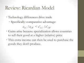
Review: Ricardian Model. Technology differences drive trade Specifically: comparative advantage: a LC / a LW < a * LC /a * LW Gains arise because specialization allows countries to sell their good at a higher (relative) price

Review: Ricardian Model
E N D
Presentation Transcript
Review: Ricardian Model • Technology differences drive trade • Specifically: comparative advantage: aLC/aLW < a*LC/a*LW • Gains arise because specialization allows countries to sell their good at a higher (relative) price • This extra income can then be used to purchase the goods they don’t produce.
Preview • Introduction • The Specific Factors Model • International Trade in the Specific Factors Model • Income Distribution and the Gains from Trade • Political Economy of Trade: A Preliminary View • Summary
Introduction • If trade is so good for the economy, why is there such opposition? To understand the politics of trade we have to look not just at the welfare of a country as a whole, but at its income distribution. • Two main reasons why international trade has strong effects on the distribution of income within a country (in the short run): • Resources cannot move immediately or costlessly from one industry to another. • Industries differ in the factors of production they demand.
The Specific Factors Model • The specific factors model(developed by Paul Samuelson and Ronald Jones) allows trade to affect income distribution. • Assumptions of the model: • Two goods, cloth and food. • Three factors of production: labor (L), capital (K) and land (T for terrain). • Focus on gains/losses to these factors • Perfect competition prevails in all markets.
The Specific Factors Model (cont.) • Cloth produced using capital (K) and labor (L) • (but not land). • Food produced using land (T) and labor • (but not capital). • Labor is a mobile factor that can move between sectors. • Land and capital are both specific factors used ONLY in the production of one good.
The Specific Factors Model (cont.) • Note: The distinction between specific and mobile factors is not a sharp line. It is a question of the speed of adjustment, with factors being more specific the longer it takes to redeploy them between industries. • Labour is certainly a less specific factor than most kinds of capital!
The Specific Factors Model (cont.) • How much of each good does the economy produce? • The production function for cloth gives the quantity of cloth that can be produced given any input of capital and labor: QC = QC (K, LC) • QC is the output of cloth • K is the capital stock • LCis the labor force employed in cloth
The Specific Factors Model (cont.) • The production function for food gives the quantity of food that can be produced given any input of land and labor: QF= QF (T, LF) • QF is the output of food • T is the supply of land • LF is the labor force employed in food For the economy as a whole, the labor employed must be equal to the total labor supply: Lc + LF = L
Production Possibilities Given that only labor can be used in both sectors, to analyze the economy’s production possibilities, we need to ask: • How does the economy’s mix of output change as labor is shifted from one sector to the other? We first represent the production functions and then we put them together to derive the PPF When labor moves from food to cloth, food production falls while output of cloth rises.
Production Possibilities (cont.) • The shape of the production function reflects the law of diminishing marginal returns. • Adding one worker to the production process (without increasing the amount of capital) means that each worker has less capital to work with. • Next, define the marginal product of labor, MPL (the slope of the function),which is the increase in output that corresponds to an extra unit of labor. • Note: We defined this as 1/aL in the Ricardian model
Production Possibilities (cont.) • For the economy as a whole, the total labor employed in cloth and food must equal the total labor supply: LC+ LF = L • Use these equations to derive the production possibilities frontier of the economy (that shows what the economy is capable of producing. In our case how much food it can produce for any given output of cloth and viceversa)
The Production Possibility Frontier in the Specific Factors Model
Production Possibilities (cont.) • Why is the production possibilities frontier curved? • Diminishing returns to labor in each sector: If LC rises, the MPLC in cloth falls; correspondingly, as LF falls, the MPLF in food raises. • Opportunity cost of cloth in terms of food is the slope of the production possibilities frontier. The opportunity cost of producing one more yard of cloth is MPLF/MPLC pounds of food. Recall this is same as unit labor costs from Ricardianmodel!
Prices, Wages and Labor Allocation • How much labor is employed in each sector? • Need to look at supply and demand in the labor market. The demand for labor in each sector depends on the price of output and the wage rate. The wage rate depends on the combined demand for labor by food and cloth producers.
Prices, Wages, and Labor Allocation (cont.) • Price (of labor) is set through the competitive labor market. • Profit maximizing employers will demand labor up to the point where the value produced by an additional person-hour equals the cost of employing that hour • The demand curve for labor in the cloth sector: MPLCx PC = w • The demand curve for labor in the food sector: MPLFx PF = w
Prices, Wages, and Labor Allocation (cont.) • Further: the two sectors must pay the same wage because labor can move between sectors. • If the wage were higher in the cloth sector, workers would move! Representing the two labor demand curves in a diagram we can see how the wage rate and employment in each sector are determined given the prices of cloth and food
http://www.nytimes.com/2013/01/13/sunday-review/americas-productivity-climbs-but-wages-stagnate.html?smid=fb-share&_r=2&http://www.nytimes.com/2013/01/13/sunday-review/americas-productivity-climbs-but-wages-stagnate.html?smid=fb-share&_r=2&
Prices, Wages, and Labor Allocation (cont.) • This is equivalent to saying: • At the production point, the production possibility frontier must be tangent to a line whose slope is: MPLF/MPLC = PC/PF
Summary So Far… • What are the “specific factors” in this model? • What role do specific factors play in this model so far? • Why do they need to be “specific”?
Summary So Far… • Concave Production Possibility Frontier • Diminishing marginal returns • Downward sloping Labor Demand functions • Unique equilibrium wage
Prices, Wages, and Labor Allocation (cont.) • What happens to the allocation of labor and the distribution of income when the prices of food and cloth change? • Two cases: • An equal proportional change in prices • A change in relative prices
Prices, Wages, and Labor Allocation (cont.) • When both prices change in the same proportion, no real changes occur. • The wage rate (w) rises in the same proportion as the prices, so real wages are unaffected. • The real incomes of capital owners and landowners also remain the same. • To see this note that price equals marginal cost.
An Equal-Proportional Increase in the Prices of Cloth and Food
Prices, Wages, and Labor Allocation (cont.) Let’s consider now the effect of a price change that does affect relative prices. • When only PC rises, labor shifts from the food sector to the cloth sector and the output of cloth rises while that of food falls. • The wage rate (w) does not rise as much as PC • The marginal product of labor in that sector falls.
Response of Output to a Change in the Relative Price of Cloth
Prices, Wages, and Labor Allocation (cont.) • What is the economic effect of this price increase on the incomes of the following three groups? • Workers, owners of capital, and owners of land
Prices, Wages, and Labor Allocation (cont.) • Owners of capital are definitely better off. Why? • Landowners are definitely worse off. Why? • Workers: cannot say whether workers are better or worse off: • Depends on the relative importance of cloth and food in workers’ consumption. • It’s possible workers are better off if their relative consumption of _____ is quite high.
International Trade in the Specific Factors Model • Trade and Relative Prices For trade to take place, a country must face a world relative price that is different from the relative price that would prevail in the absence of trade. • Countries may differ not only in terms of labor, but in terms of other resources: land and capital. • There are no differences in relative demand across countries.
When the economy is open to trade, the relative price of cloth is determined by the relative supply and demand for the world. The increase in the relative price induces the economy to produce relatively more cloth. • At the same time, consumers respond to the higher relative price of cloth by demanding relatively more food. At the world relative price the economy thus exports cloth and import foods.
International Trade in the Specific Factors Model (cont.) • Gains from Trade • Without trade, the economy’s output of a good must equal its consumption. The consumption of the economy would have to be a point on the production possibility frontier. Ex. Point 2 in the graph. • A trading economy might consume more of both goods than it would have in absence of trade. The budget constraint represents all the possible combinations of food and cloth that the country could consume given the world relative price of cloth. The budget constraint with trade lies above the production possibilities frontier. Trade expands the economy’ s choices.
The Budget Constraint for a Trading Economy and Gains from Trade
Income Distribution and the Gains from Trade • Factor prices: • Trade benefits the factor that is specific to the export sector of each country, but hurts the factor that is specific to the import-competing sectors. • Trade has ambiguous effects on mobile factors.
Income Distribution and the Gains from Trade (cont.) • Trade benefits a country by expanding choices. • Possible to redistribute income so that everyone gains from trade. • Those who gain from trade could compensate those who lose and still be better off themselves. • Most economists strongly favor free trade.
Trade and Unemployment • Trade shifts jobs from import-competing to export sector. • Process not instantaneous – some workers will be unemployed. • How much unemployment can be traced back to trade? • From 1996 to 2008, only about 2.5% of involuntary displacements stemmed from import competition or plants moved overseas.
Trade and Unemployment (cont.) • There is no obvious correlation between unemployment rate and imports relative to GDP for the U.S.
Unemployment and Import Penetration in the U.S. Source: US Bureau of Economic Analysis for imports and US Bureau of Labor Studies for unemployment.
International Labor Mobility • Whenever international migration is possible, workers will want to move from the low wage to the high wage country*. • Assumptions: • Two countries and one good • Two factors of production: labor (mobile) and land (immobile) Since there is only one good there is no reason to trade it. Trade in labor services between the two countries is possible, with workers moving in search of higher wages. *We assume that workers’ tastes are similar so that location decisions are based on wage differentials
International Labor Mobility (cont.) Horizontal axis: Total world labor force The two marginal labor curves represent production of the same good in different countries Vertical axis: real wages (the wage divide by the price of the unique good in each country)
International Labor Mobility (cont.) • Convergence of real wage rates. Real wage rise in Home and fall in Foreign • Increase of the world output as a whole. Foreign’s output increases, while Home’s output decreases. Foreign’s gain is higher than Home’s loss, by an amount equal to the colored area ABC in the figure. • Some people are hurt by the change. Those who originally worked in Home receive a higher real wage, while those who worked in Foreign a lower. Landowners in Foreign benefit from the larger labor supply, but landowners in Home are made worse off.
Summary Questions • Who gains from an increase in the relative price of food? Who loses? • When would workers gain from this increase?
Showing that Output Is Equal to the Area Under the Marginal Product Curve
