Schema Refinement and Normal Forms
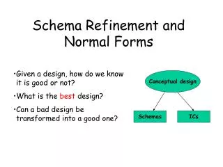
Schema Refinement and Normal Forms. Review: Database Design. Requirements Analysis user needs; what must database do? Conceptual Design high level description (often done w/ER model) Logical Design translate ER into DBMS data model Schema Refinement consistency, normalization

Schema Refinement and Normal Forms
E N D
Presentation Transcript
Review: Database Design • Requirements Analysis • user needs; what must database do? • Conceptual Design • high level description (often done w/ER model) • Logical Design • translate ER into DBMS data model • Schema Refinement • consistency, normalization • Physical Design - indexes, disk layout • Security Design - who accesses what
Design Steps • Step (3) to step (4) is based on a “design theory” for relations and is called “normalization”. It is important for two reasons: • Automatic mappings from ER to relations may not produce the best relational design possible. • Database designers may go directly from (1) to (3), in which case, the relational design can be really bad.
Informal guidelines • Semantics of the attributes • easy to explain relation • doesn’t mix concepts • Reducing the redundant values in tuples • Choosing attribute domains that are atomic • Reducing the null values in tuples • Disallowing spurious tuples
1. Semantics of Attributes • Semantics of attributes specify how to interpret the attributes values stored in a tuple of the relation. • In other words, how the attributes’ values in a tuple are related to one another. Guideline 1: • Design a relation schema so that it is easy to explain its meaning. • Do not combine attributes from multiple entity types and relationship types into a single relation.
2. Null Values • If many of the attributes do not apply to all tuples in the relation, we end up with many null values (no value) in those tuples. • This leads to wasted space and misunderstandings. Guideline 2: • As much as possible, avoid placing attributes in a relation whose values may frequently be null. • If nulls are unavoidable, make sure that they apply in exceptional cases, and do not apply to the majority of tuples in the relation.
3. Spurious Tuples • Additional tuples that were not in the original relation are called spurious tuples because they represent spurious or wrong information that is not valid. • This is called the lossless join property. Guideline 3: • Design relation schemas so that they can beJOINed (with equality condition on attributes that are either primary keys or foreign keys) in a way that guarantees that no spurious tuples are generated.
CustomerID Title Date Price Kind 0001 True Lies 04-19-2002 3.25 D 0002 True Lies 04-21-2002 3.25 D 0001 The Lion King 04-19-2002 4.00 C 0003 The Lion King 04-19-2002 4.00 C 0001 Henry V 04-18-2002 1.75 D 3. Spurious Tuples cont.
Title Price Kind True Lies 3.25 D The Lion King 3.25 C Henry V 1.75 D CustomerID Title Price Kind Date 0001 True Lies 3.25 D 04-19-2002 0002 True Lies 3.25 D 04-21-2002 0001 The Lion King 3.25 C 04-19-2002 0003 The Lion King 3.25 C 04-19-2002 0001 Henry V 1.75 D 04-18-2002 0002 The Lion King 3.25 D 04-21-2002 0003 True Lies 3.25 C 04-19-2002 3. Spurious Tuples cont. Bad Relational Schema: CustomerID Price Date 0001 3.25 04-19-2002 0002 3.25 04-21-2002 0003 3.25 04-19-2002 0001 1.75 04-18-2002 The Join Of the Above 2 Relations
Title Price Kind True Lies 3.25 D The Lion King 3.25 C Henry V 1.75 D CustomerID Title Date 0001 True Lies 04-19-2002 0002 True Lies 04-21-2002 CustomerID Title Price Kind Date 0001 The Lion King 04-19-2002 0001 True Lies 3.25 D 04-19-2002 0003 The Lion King 04-19-2002 0002 True Lies 3.25 D 04-21-2002 0001 Henry V 04-18-2002 0001 The Lion King 3.25 C 04-19-2002 0003 The Lion King 3.25 C 04-19-2002 0001 Henry V 1.75 D 04-18-2002 3. Spurious Tuples cont. Good Relational Schema: The Join Of the Above 2 Relations
CustomerID Title Date Price Kind 0001 True Lies 04-19-2002 3.25 D 0002 True Lies 04-21-2002 3.25 D 0001 The Lion King 04-19-2002 4.00 C 0003 The Lion King 04-19-2002 4.00 C 0001 Henry V 04-18-2002 1.75 D 4. Reducing Redundancies cont. Modification Anomalies: • Insertion Anomaly: • Cannot insert information about a film if it has not been rented yet. • Update Anomaly: • Updating the rental price for “True Lies” to $4, requires changing it in several typles (if not, it will cause inconsistencies). • Deletion Anomaly: • Deleting the rental information will cause the film information to disappear.
4. Reducing Redundancies • Redundancies in a relation schema result in: • Waste of space • Potential for inconsistent data (loss of data integrity) • Potential for modification anomalies (unusual behavior): • Insertion anomalies • Update anomalies • Deletion anomalies Guideline 4: • Design the relation schemas so that no insertion, modification, or modification anomalies occur.
Integrity constraints, in particularfunctional dependencies, can be used to identify schemas with such problems and to suggest refinements. • Decomposition should be used judiciously: • Is there reason to decompose a relation? • What problems (if any) does the decomposition cause?
Q1)answered by applying various Normal forms Q2)answered by properties of decomposition that interests us are lossless-join ( enables us to recover any instance of the decomposed relation from corresponding instances of the smaller relations) dependency-preservation ( enables us to enforce any constraint on the original relation by simply enforcing some constraints on each of the smaller relations. We do not have to perform join of smaller relation to check if a constraint on original relation is violated.
From Performance point of view If queries over the original relation are common then decomposing is not acceptable In some cases the decomposition is improves performance when queries and updates examine only decomposed relations.
A BAD Relational Schema An Improved Schema
What’s a Good Design? • Three properties: • No anomalies. • Can reconstruct all original information. • Ability to check all FDs within a single relation. • Role of FDs in detecting redundancy: • Consider a relation R with 3 attributes, ABC. • No FDs hold: There is no redundancy here. • Given A B: Several tuples could have the same A value, and if so, they’ll all have the same B value!
Decomposition of a Relation Scheme • Suppose that relation R contains attributes A1 ... An. A decompositionof R consists of replacing R by two or more relations such that: • Each new relation scheme contains a subset of the attributes of R (and no attributes that do not appear in R), and • Every attribute of R appears as an attribute of one of the new relations. • Intuitively, decomposing R means we will store instances of the relation schemes produced by the decomposition, instead of instances of R. • E.g., Can decompose SNLRWH into SNLRH and RW.
Functional Dependency • A functional dependency (FD) is a constraint between two sets of attributes in relation R. • It is denoted by: X Y • Reads: • Y is functionally dependent on X • X (functionally) determines Y • Means: • If two tuples in R agree on their X-value, they must necessarily agree on their Y-value.
Functional Dependencies (FDs) • A functional dependencyX Y holds over relation R if, for every allowable instance r of R: • i.e., given two tuples in r, if the X values agree, then the Y values must also agree. (X and Y are sets of attributes.) • K is a key for relation R if: 1. K determines all attributes of R. 2. For no proper subset of K is (1) true. • If K satisfies only (1), then K is a superkey. • K is a candidate key for R means that K R • However, K R does not require K to be minimal!
Functional Dependencies (FDs) • A functional dependencyX Y holds over relation schema R if, for every allowable instance r of R: t1 r, t2 r, pX(t1) = pX(t2) implies pY(t1) = pY(t2) (where t1 and t2 are tuples;X and Y are sets of attributes) • In other words: X Y means Given any two tuples in r, if the X values are the same, then the Y values must also be the same. (but not vice versa) • Read “” as “determines”
EMP_PROJ(SSN, PNUMBER, HOURS, ENAME , PNAME, PLOCATION) FD Diagram FD Examples cont. Can Assert the FDs SSN ENAME PNUMBER { PNAME, PLOCATION } { SSN, PNUMBER } HOURS
Example • Consider relation Hourly_Emps: • Hourly_Emps (ssn, name, lot, rating, hrly_wages, hrs_worked) • FD is a key: • ssn is the key • S SNLRWH • FDs give more detail than the mere assertion of a key. • rating determines hrly_wages • R W
FD’s Continued • An FD is a statement about all allowable relations. • Must be identified based on semantics of application. • Given some instance r1 of R, we can check if r1 violates some FD f, but we cannot determine if f holds over R. • FDs are a generalization of keys.
FD T/F AB C is equivalent to {A, B} C Try This One Assuming that all the FDs in the relation are apparent in the following instance of the relation: A B F A C T B A F B C F C A T C B F AB C T AC B F BC A T
R (SID, CourseID, TotalCreditHours, Grade , SName, Status) Can Assert the FDs … and This One SID { SName, TotalCreditHours, Status } { SID, CourseID } Grade TotalCreditHours Status
Notes about FDs • Functional dependencies are constraints that hold on the whole relation R, not on any particular instance of the relation. • An FD X Y is trivial if YX (subset) Examples: • StuID StuID • { StuID, CourseID } CourseID • X Y does not mean Y X (an FD is not reversible)
Notes about FDs cont. • The left-hand-side (LHS) of any FD X Y (Xin this case) is called a determinant. • Even though we can write X YZ (standard form), you should always remember that this is TWOFDs in one: X Y and X Z (canonical form). • We can write the above formally as: X YZ|={ X Y , X Z } ( |=denotes “logical implication”)
R (SID, CourseID, TotalCreditHours, Grade , SName, Status) F = {SID { SName, TotalCreditHours, Status }, { SID, CourseID } Grade TotalCreditHours Status} Notes about FDs cont. • We denote by Fthe set of functional dependencies that are specified on a relation schema R.
R (SID, CourseID, TotalCreditHours, Grade , SName, Status) SID SName {SID, CourseID} Grade {SID, CourseID} SName {SID, CourseID} Status Notes about FDs cont. • If X Y is an FD that holds in R, we say that Y is fully FD on X if removal of any attribute from X means that the FD does not hold any more; otherwise, we say Y is partially FD on X. • Notice that if X is a single attribute, then for sure Y is fully FD on X. SName is fully FD onSID Grade is fully FD on {SID, CourseID} SName is NOT fully FD on {SID, CourseID} Status is NOT fully FD on {SID, CourseID}
Reasoning About FDs • Given some FDs, we can usually infer additional FDs: • ssn did, did lot implies ssn lot • An FD f is implied bya set of FDs F if f holds whenever all FDs in F hold. • F+ = closure of F is the set of all FDs that are implied by F. • Armstrong’s Axioms (X, Y, Z are sets of attributes): • Reflexivity: If Y X, then X Y • Augmentation: If X Y, then XZ YZ for any Z • Transitivity: If X Y and Y Z, then X Z • These are sound and completeinference rules for FDs!
FD Inference Rules IR1 (Reflexivity): X Y |= X Y • X is superset of Y • The trivial dependency rule (e.g.AB B); useful for derivations. IR2 (Augmentation): X Y |= XZ YZ • If a dependency holds, then we can freely expand its left hand side. IR3 (Transitivity):X Y, Y Z |= X Z • The most powerful inference rule; useful in multi-step derivations.
FD Inference Rules cont. Armstrong inference rules (also called Armstrong’s Axioms) are: • Sound: meaning that given a set of FDs F specified on a relation schema R, any FD that we can infer from F by using IR1 through IR3 holds on every relation state (instance) of R that satisfies the dependencies in F. • Complete: meaning that using IR1 through IR3 repeatedly to infer FDs, until no more FDs can be inferred, results in the complete set of all possible FDs that can be inferred from F (closure of F, denoted as F+).
IR Proofs Prove or Disprove: X YZ|= X Y and X Z (decomposition or projective rule IR4) X YZ(given) YZ Y(using IR1 and knowing that YZ Y) X Y(using IR3 on 1 and 2)
Reasoning About FDs (Cont.) • Couple of additional rules (that follow from AA): • Union IR5: If X Y and X Z, then X YZ • Proof of Union: • X Y (given) • X XY (augmentation using X) • X Z (given) • XY YZ (augmentation) • X YZ (transitivity)
IR Proofs Prove or Disprove: X Y, WY Z |= WX Z (pseudotransitive rule IR6) X Y(given) WY Z(given) WX WY(using IR2 on 1 by augmenting with W) WX Z(using IR3 (transitivity) on 3 and 2)
Reasoning About FDs • Computing the closure of a set of FDs can be expensive. (Size of closure is exponential in # attrs!) • Typically, we just want to check if a given FD X Y is in the closure of a set of FDs F. An efficient check: • Compute attribute closureof X (denoted X+) wrt F: • Set of all attributes A such that X A can be inferred using the Armstrong Axioms • There is a linear time algorithm to compute this. • Check if Y is in X+ • Does F = {A B, B C, C D E } imply A E? • i.e, is A E in the closure F+ ? Equivalently, is E in A+ ?
Finding All Implied FDs • Motivation: Suppose we have a relation ABCD with some FDs F. If we decide to decompose ABCD into ABC and AD, what are the FDs for ABC, AD? • Example: F = AB C, C D, D A. It looks like just AB C holds in ABC, but in fact C A follows from F and applies to relation ABC. • Problem is exponential in worst case. • Algorithm to find F+: • For each set of attributes X of R, compute X+.
X+ := X repeat oldX+ := X+ for each FD Y Z in F do if Y X+ then X+ := X+ Z until oldX+ = X+ Closure of Attributes • Given a set of FDs F in relation R, the set of all the attributes that can be determined (directly or indirectly) from a given attribute (or set of attributes) X is called the closure of X, denoted by X+ • X+ can be determined using the simple algorithm: