Consider the graphs of f ( x ) = x – 1 and f ( x ) = ln x .

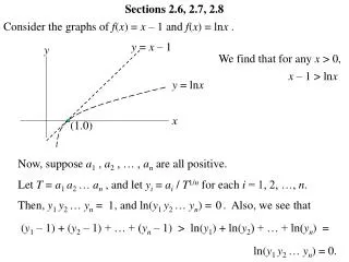
1. Sections 2.6, 2.7, 2.8 Consider the graphs of f(x) = x– 1 and f(x) = lnx . y = x– 1 y We find that for any x > 0, x – 1 > lnx y = lnx x (1.0) Now, suppose a1 , a2 , … , an are all positive. Let T = a1 a2 … an , and let yi = ai / T1/n for each i = 1, 2, …, n. Then, y1 y2 … yn = , and ln(y1 y2 … yn) = . Also, we see that 1 0 (y1– 1) + (y2– 1) + … + (yn– 1) > ln(y1) + ln(y2) + … + ln(yn) = ln(y1 y2 … yn) = 0.

2. We now have that (y1– 1) + (y2– 1) + … + (yn– 1) > 0  y1 + y2 + … + yn ——————— > 1  n y1 + y2 + … + yn > n a1 + a2 + … + an ——————— > 1  T1/nn a1 + a2 + … + an ——————— > (a1a2…an)1/n n In Appendix III (page 394), find the definition of the arithmetic mean and the geometric mean. Then observe that we have proven that that the arithmetic mean must always be greater than or equal to the geometric mean (assuming of course only positive values).

3. Amounts $500, $800, and $1000 are to be paid at respective times 3 years from today, 5 years from today, and 11 years from today. Suppose we would like to find the number of years t from today when one single payment of $500 + $800 + $1000 = $2300 would be equivalent to the individual payments made separately. If the rate of interest per annum is known to be i, then v = 1 / (1 + i), and the equation of value is 2300vt = 500v3 + 800v5 + 1000v11 In general, suppose amounts s1 , s2 , … , sn are to be paid at respective times t1 , t2 , … , tn . Also suppose we would like to find the time t when one single payment of s1 + s2 + … + sn would be equivalent to the individual payments made separately. If v = 1 / (1 + i) is known, then the equation of value is t1t2tn (s1 + s2 + … + sn)vt = s1v + s2v + … + snv (One of the homework assignments will have you find an exact formula for the unknown value of t.)

4. t1t2tn (s1 + s2 + … + sn)vt = s1v + s2v + … + snv With the exact t, this is the true present value for the equivalent single payment. An approximate value of t can be obtained from the method of equated time. This method estimates t with s1t1 + s2t2 + … + sntn t = ————————— s1 + s2 + … + sn With the approximation t, the estimated present value for the equivalent single payment is t (s1 + s2 + … + sn)v In order to discover an interesting property about how the exact value of t and the estimate t compare, let us imagine that we have a list of numbers where s1 of the numbers are equal to v , s2 of the numbers are equal to v , etc. t1 t2

5. In order to discover an interesting property about how the exact value of t and the estimate t compare, let us imagine that we have a list of numbers where s1 of the numbers are equal to v , s2 of the numbers are equal to v , etc. t1 t2 s1t1 + s2t2 + … + sntn ————————— s1 + s2 + … + sn t Then v can be written as v = 1 —————— s1 + s2 + … + sn From Appendix III, we see that this is the geometric mean of the list of numbers. s1t1 s2t2 sntn v v … v This is the product of the list of numbers. t1t2tn s1v + s2v + … + snv —————————— s1 + s2 + … + sn t and v can be written as From Appendix III, we see that this is the arithmetic mean of the list of numbers. This is the average of the list of numbers.

6. Since the arithmetic mean of positive numbers must always be larger than the geometric mean, we have that t t v > v t1t2tn s1v + s2v + … + snv —————————— s1 + s2 + … + sn t > v t t1t2tn s1v + s2v + … + snv > (s1 + s2 + … + sn)v We now see that the true present value (on the left) will always be larger than the estimated present value (on the right). Consequently, the estimated time t from the method of equated time must be an overestimation.

7. Amounts $500, $800, and $1000 are to be paid at respective times 3 years from today, 5 years from today, and 11 years from today. The effective rate of interest is 4.5% per annum. (a) (b) Use the method of equated time to find the number of years t from today when one single payment of $500 + $800 + $1000 = $2300 would be equivalent to the individual payments made separately. s1t1 + s2t2 + … + sntn t = ————————— = s1 + s2 + … + sn (500)(3) + (800)(5) + (1000)(11) ————————————— = 2300 7.174 years Find the exact number of years t from today when one single payment of $500 + $800 + $1000 = $2300 would be equivalent to the individual payments made separately. With v = 1 / (1 + 0.045), the equation of value is 2300vt = 500v3 + 800v5 + 1000v11 500v3 + 800v5 + 1000v11 vt = —————————— = 2300 0.73752 t = 6.917 years

8. Given a particular rate of interest, how long will it take an investment to double? By solving (1 + i)n = 2, we find the exact solution n = ln(2) ——— ln(1 + i) 0.6931 ——— = ln(1 + i) 0.6931 i ——— ——— , i ln(1 + i) Observe that n 0.72 —— = i 72 —— . 100i and when i = 0.08 in the second factor, we have n This is called the rule of 72, and it gives amazingly accurate results for a wide range of interest rates! (See Table 2.1 on page 47 of the text.)

9. Suppose $2000 is invested at a rate of 7% compounded semiannually. (a) (b) (c) Find the length of time for the investment to double by using the exact formula. t = years  2000(1.035)2t = 4000  t = 10.074 years Find the length of time for the investment to double by using the rule of 72. 72/3.5 = 20.571 half years t = 10.286 years Find the length of time for the investment to double by using the interest tables. Interpolating from the tables, we obtain (2 – 1.98979) 20 + (21 – 20) ————————— = 20.147 half-years = (2.05943 – 1.98979) 10.073 years

10. Suppose $2000 is invested at a rate of 7% compounded semiannually. (d) (e) Find the length of time for the investment to be worth $3000 by using the exact formula. t = years  2000(1.035)2t = 3000  t = 5.893 years Find the length of time for the investment to be worth $3000 by using the interest tables. Interpolating from the tables, we obtain (2 – 1.45997) 11 + (12 – 11) ————————— = 11.514 half-years = (1.51107 – 1.45997) 5.756 years

11. Suppose it is the rate of interest i that is unknown in an equation of value. There are four different methods to be considered in solving for i. Depending on the type of situation, one method may be better suited than another. At what interest rate convertible semiannually would $500 accumulate to $800 in 4 years? When a single payment is involved, the method that works best is to solve for i directly in the equation of value (using exponential and logarithmic functions). 500(1 + j)8 = 800 1 + j = (8/5)1/8 j = (8/5)1/8 – 1 = 0.0605 i(2) = 2j = (2)(0.0605) = 0.0121 = 12.1%

12. At what effective interest rate would the present value of $1000 at the end of 3 years plus $2000 at the end of 6 years be equal to $2700? When multiple payments are involved, the equation of value is generally a polynomial, and the method to solve for i is one for obtaining the roots of a polynomial. Sometimes this can be done using the quadratic formula. 1000v3 + 2000v6 = 2700 2000v6 + 1000v3– 2700 = 0 20v6 + 10v3– 27 = 0 We are only interested in v > 0, and the only positive root from the quadratic formula is v3 = , from which we obtain v = 0.9385 0.9791. v = 1 / (1 + i) = 0.9791 i = 0.02145

13. Look at Example 2.9 (pages 49-50) in the textbook. When multiple payments are involved, the equation of value is generally a polynomial, and the method to solve for i is one for obtaining the roots of a polynomial. If this cannot be done using the quadratic formula, then some trial an error together with interpolation in the interest tables can be used. Look at Example 2.10 (pages 50-51) in the textbook. When multiple payments are involved, the equation of value is generally a polynomial, and the method to solve for i is one for obtaining the roots of a polynomial. For a more accurate answer than one obtained from interpolation in the interest tables, an iterative procedure can be used. The use of a computer generally makes an iterative procedure much easier to use. Use the Excel file Interest_Solver to find the solution in Example 2.10 as follows:

14. Type the formula =1000*(1+j)^20+2000*(1+j)^14-5000 in cell A5. Select options Tools > Solver to solve the equation of value as indicated below (and if necessary, first use options Tools > Add-Ins) Section 2.8 of the textbook discusses some of the ambiguous interpretations of words used in the “real world” versus the precise meanings used in mathematics.