CS 267: Applications of Parallel Computers Unstructured Multigrid for Linear Systems
770 likes | 938 Vues
CS 267: Applications of Parallel Computers Unstructured Multigrid for Linear Systems. James Demmel Based in part on material from Mark Adams (www.columbia.edu/~ma2325) www.cs.berkeley.edu/~demmel/cs267_Spr07. Recall Big Idea used several times in course. To solve a hard problem,

CS 267: Applications of Parallel Computers Unstructured Multigrid for Linear Systems
E N D
Presentation Transcript
CS 267: Applications of Parallel ComputersUnstructured Multigrid for Linear Systems James Demmel Based in part on material from Mark Adams (www.columbia.edu/~ma2325) www.cs.berkeley.edu/~demmel/cs267_Spr07 CS267 Guest Lecture
Recall Big Idea used several times in course • To solve a hard problem, • Use a coarse approximation, which is solved recursively by coarser ones • Depends on coarse approximation being accurate enough if we are far enough away • “Coarse” means small to represent, so fast to compute or communicate • Multilevel Graph Partitioning (METIS): • Replace graph to be partitioned by a coarser graph, obtained via Maximal Independent Set • Given partitioning of coarse grid, refine using Kernighan-Lin • Barnes-Hut and Fast Multipole Method for computing gravitational forces on n particles in O(n log n) time: • Approximate particles in box by total mass, center of gravity • Good enough for distant particles; for close ones, divide box recursively • Solving Poisson equation on mesh using Multigrid • Approximate low frequency part of solution using coarse mesh • How general is this idea? CS267 Guest Lecture
“BR” tire: compute displacement during rolling Source: Mark Adams, PPPL CS267 Guest Lecture
Displacement history Source: Mark Adams, PPPL CS267 Guest Lecture
Source of Unstructured Finite Element Mesh: Vertebra Study failure modes of trabecular Bone under stress Source: M. Adams, H. Bayraktar, T. Keaveny, P. Papadopoulos, A. Gupta CS267 Guest Lecture
Methods: FE modeling Mechanical Testing E, yield, ult, etc. Source: Mark Adams, PPPL 3D image FE mesh 2.5 mm cube 44 m elements Micro-Computed Tomography CT @ 22 m resolution Up to 537M unknowns CS267 Guest Lecture
Outline • Recall Poisson Equation on regular mesh • Recall solution by Multigrid • Geometric Multigrid • Algebraic Multigrid • Software framework • Numerical examples CS267 Guest Lecture
Graph and “stencil” -1 2 -1 T = Poisson’s equation in 1D: 2u/x2 = f(x) 2 -1 -1 2 -1 -1 2 -1 -1 2 -1 -1 2 CS267 Guest Lecture
2D Poisson’s equation • Similar to the 1D case, but the matrix T is now • 3D is analogous Graph and “stencil” 4 -1 -1 -1 4 -1 -1 -1 4 -1 -1 4 -1 -1 -1 -1 4 -1 -1 -1 -1 4 -1 -1 4 -1 -1 -1 4 -1 -1 -1 4 -1 -1 4 -1 T = -1 CS267 Guest Lecture
Multigrid Overview • Basic Algorithm: • Replace problem on fine grid by an approximation on a coarser grid • Solve the coarse grid problem approximately, and use the solution as a starting guess for the fine-grid problem, which is then iteratively updated • Solve the coarse grid problem recursively, i.e. by using a still coarser grid approximation, etc. • Success depends on coarse grid solution being a good approximation to the fine grid CS267 Guest Lecture
smoothing Finest Grid First Coarse Grid Error on fine and coarse grids Restriction (R) CS267 Guest Lecture
Multigrid uses Divide-and-Conquer in 2 Ways • First way: • Solve problem on a given grid by calling Multigrid on a coarse approximation to get a good guess to refine • Second way: • Think of error as a sum of sine curves of different frequencies • Same idea as FFT-based solution, but not explicit in algorithm • Replacing value at each grid point by a certain weighted average of nearest neighbors decreases the “high frequency error” • Multigrid on coarse mesh decreases the “low frequency error” CS267 Guest Lecture
Multigrid Sketch in 2D • Consider a 2m+1 by 2m+1 grid in 2D • Let P(i) be the problem of solving the discrete Poisson equation on a 2i+1 by 2i+1 grid in 2D • Write linear system as T(i) * x(i) = b(i) • P(m) , P(m-1) , … , P(1) is sequence of problems from finest to coarsest Need to generalize this to unstructured meshes / matrices CS267 Guest Lecture
Multigrid Operators • For problem P(i) : • b(i) is the RHS and • x(i) is the current estimated solution • All the following operators just average values on neighboring grid points (so information moves fast on coarse grids) • The restriction operator R(i) maps P(i) to P(i-1) • Restricts problem on fine grid P(i) to coarse grid P(i-1) • Uses sampling or averaging • b(i-1)= R(i) (b(i)) • The interpolation operator In(i-1) maps approx. solution x(i-1) to x(i) • Interpolates solution on coarse grid P(i-1) to fine grid P(i) • x(i) = In(i-1)(x(i-1)) • The solution operator S(i) takes P(i) and improves solution x(i) • Uses “weighted” Jacobi or SOR on single level of grid • x improved (i) = S(i) (b(i), x(i)) • both live on grids of size 2i-1 Need to generalize these to unstructured meshes / matrices CS267 Guest Lecture
Multigrid V-Cycle Algorithm Function MGV ( b(i), x(i) ) … Solve T(i)*x(i) = b(i) given b(i) and an initial guess for x(i) … return an improved x(i) if (i = 1) compute exact solution x(1) of P(1)only 1 unknown return x(1) else x(i) = S(i) (b(i), x(i)) improve solution by damping high frequency error r(i) = T(i)*x(i) - b(i) compute residual d(i) = In(i-1) ( MGV( R(i) ( r(i) ), 0 ))solveT(i)*d(i) = r(i)recursively x(i) = x(i) - d(i) correct fine grid solution x(i) = S(i) ( b(i), x(i) ) improve solution again return x(i) CS267 Guest Lecture
Why is this called a V-Cycle? • Just a picture of the call graph • In time a V-cycle looks like the following CS267 Guest Lecture
The Solution Operator S(i) - Details • The solution operator, S(i), is a weighted Jacobi • Consider the 1D problem • At level i, pure Jacobi replaces: x(j) := 1/2 (x(j-1) + x(j+1) + b(j) ) • Weighted Jacobi uses: x(j) := 1/3 (x(j-1) + x(j) + x(j+1) + b(j) ) • In 2D, similar average of nearest neighbors CS267 Guest Lecture
Weighted Jacobi chosen to damp high frequency error Initial error “Rough” Lots of high frequency components Norm = 1.65 Error after 1 Jacobi step “Smoother” Less high frequency component Norm = 1.06 Error after 2 Jacobi steps “Smooth” Little high frequency component Norm = .92, won’t decrease much more CS267 Guest Lecture
The Restriction Operator R(i) - Details • The restriction operator, R(i), takes • a problem P(i) with RHS b(i) and • maps it to a coarser problem P(i-1) with RHS b(i-1) • In 1D, average values of neighbors • xcoarse(i) = 1/4 * xfine(i-1) + 1/2 * xfine(i) + 1/4 * xfine(i+1) • In 2D, average with all 8 neighbors (N,S,E,W,NE,NW,SE,SW) CS267 Guest Lecture
Interpolation Operator In(i-1): details • The interpolation operator In(i-1), takes a function on a coarse grid P(i-1) , and produces a function on a fine grid P(i) • In 1D, linearly interpolate nearest coarse neighbors • xfine(i) = xcoarse(i) if the fine grid point i is also a coarse one, else • xfine(i) = 1/2 * xcoarse(left of i) + 1/2 * xcoarse(right of i) • In 2D, interpolation requires averaging with 4 nearest neighbors (NW,SW,NE,SE) CS267 Guest Lecture
Parallel 2D Multigrid • Multigrid on 2D requires nearest neighbor (up to 8) computation at each level of the grid • Start with n=2m+1 by 2m+1 grid (here m=5) • Use an s by s processor grid (here s=4) CS267 Guest Lecture
Available software • Hypre: High Performance Preconditioners for solving linear systems of equations/ • www.llnl.gov/CASC/linear_solvers • Talks at www.llnl.gov/CASC/linear_solvers/present.html • Goals • Scalability to large parallel machines • Easy to use • Multiple ways to describe system to solve • Multiple solvers to choose • PETSc: Portable Extensible Toolkit for Scientific Computation • www-unix.mcs.anl.gov/petsc/petsc-as • ACTS Collection – to find these and other tools • acts.nersc.gov CS267 Guest Lecture
Outline • Recall Poisson Equation on regular mesh • Recall solution by Multigrid • Geometric Multigrid • Algebraic Multigrid • Software framework • Numerical examples CS267 Guest Lecture
Generalizing Multigrid beyond Poisson, to unstructured meshes • Given original problem, how do we generate a sequence of coarse approximations? • For finite element problems, could regenerate matrix starting on coarser mesh • Need access to original physical problem and finite element modeling system, i.e. a lot more than just the original matrix, so it may be impossible • What does “coarse” mean, once very coarse? • Geometric Multigrid • Assume we know (x,y,z) coordinates of underlying mesh, and matrix • Generate coarse mesh points, analogous to taking every other point in regular mesh • Retriangulate to get new mesh • Use finite element shape functions on coarse mesh to project fine matrix to coarse one • Algebraic Multigrid • Don’t even have (x,y,z) coordinates, just matrix CS267 Guest Lecture
Geometric Multigrid • Need matrix, (x,y,z) coordinates of mesh points • Not minimum information (just matrix), but a little more • Based on work of Guillard, Chan, Smith • Finite element intuition • Goal is to compute function, represented by values at points • Think of approximation by piecewise linear function connecting points • Easy in 1D, need triangulated mesh in 2D, 3D uses tetrahedra • Geometric coarsening • Pick a subset of coarse points “evenly spaced” among fine points • Use Maximal Independent Sets • Try to keep important points, like corners, edges of object • Retriangulate coarse points • Try to approximate answer by piecewise linear function on new triangles • Let columns of P (“prolongator) be values at fine grid points given values at coarse ones • Generalizes Interpolation operator “In” from before • Acoarse = PT Afine P – Galerkin method CS267 Guest Lecture
Example of Geometric Coarsening CS267 Guest Lecture
Examples of meshes from geometric coarsening CS267 Guest Lecture
What can go wrong • Care needed so coarse grid preserves geometric features of fine grid • Label fine grid points as corner, edge, face, interior • Delete edges between same-labeled points in different features • Ex: delete edges between points on different faces • Keeps feature represented on coarse meshes CS267 Guest Lecture
How to coarsen carefully CS267 Guest Lecture
Algebraic Multigrid • No information beyond matrix needed • Galerkin still used to get Acoarse = PT Afine P • Prolongator P defined purely algebraically • Cluster fine grid points into nearby groups • Can use Maximal Independent Sets or Graph Partitioning • Use magnitude of entries of Afine to cluster • Associate one coarse grid node to each group • To interpolate coarse grid values to associated fine grid point, use properties of elasticity problem: • Rigid body modes of coarse grid point • Let coarse grid point have 6 dof (3 translation, 3 rotation) • Can be gotten from QR factorization of submatrix of Afine • Can also apply smoother to resulting columns of P • “Smoothed Aggregation” • Based on work of Vanek, Mandel, Brezina, Farhat, Roux, Bulgakov, Kuhn … CS267 Guest Lecture
Parallel Smoothers for Unstructured Multigrid • Weighted Jacobi • Easy to implement, hard to choose weight • Gauss-Seidel • Works well, harder to parallelize because of triangular solve • Polynomial Smoothers • Chebyshev polynomial p(Afine) • Easy to implement (just SpMVs with Afine ) • Chebyshev chooses p(y) such that • |1 - p(y) y |= min over interval [* , max] estimated to contain eigenvalues of Afine CS267 Guest Lecture
Outline • Recall Poisson Equation on regular mesh • Recall solution by Multigrid • Geometric Multigrid • Algebraic Multigrid • Software framework • Numerical examples CS267 Guest Lecture
Computational Architecture Silo DB Silo DB Silo DB Silo DB FE MeshInput File ParMetis Athena Partition to SMPs FE input file(in memory) FE input file(in memory) • Athena: Parallel FE • ParMetis • Parallel Mesh Partitioner (Univerisity of Minnesota) • Prometheus • Multigrid Solver • FEAP • Serial general purpose FE application (University of California) • PETSc • Parallel numerical libraries (Argonne National Labs) ParMetis Athena Athena File File File File FEAP FEAP FEAP FEAP Material Card pFEAP Olympus METIS METIS METIS Prometheus METIS Visualize ParMetis PETSc CS267 Guest Lecture
Outline • Recall Poisson Equation on regular mesh • Recall solution by Multigrid • Geometric Multigrid • Algebraic Multigrid • Software framework • Numerical examples • Work of Mark Adams • Scaled Speedup CS267 Guest Lecture
Scalability • Inexact Newton • CG linear solver • Variable tolerance • Smoothed aggregation AMG preconditioner • Nodal block diagonal smoothers: • 2nd order Chebyshev (add.) • Gauss-Seidel (multiplicative) 80 µm w/o shell CS267 Guest Lecture
Partitioning the Vertebra with ParMETIS CS267 Guest Lecture
80 µm w/ shell Vertebral Body With Shell • Large deformation elasticity • 6 load steps (3% strain) • Scaled speedup • ~131K dof/processor • 7 to 537 million dof • 4 to 292 nodes • IBM SP Power3 • 14 of 16 procs/node used • Up to 4088 processors • Double/Single Colony switch CS267 Guest Lecture
Computational phases • Mesh setup (per mesh): • Coarse grid construction (aggregation) • Graph processing • Matrix setup (per matrix): • Coarse grid operator construction • Sparse matrix triple product PTAP • Subdomain factorizations • Solve (per RHS): • Matrix vector products (residuals, grid transfer) • Smoothers (Matrix vector products) CS267 Guest Lecture
Linear solver iterations CS267 Guest Lecture
131K dof / proc - Flops/sec/proc .47 Teraflops - 4088 processors CS267 Guest Lecture
Sources of scale inefficiencies in solve phase CS267 Guest Lecture
Outline • Recall Poisson Equation on regular mesh • Recall solution by Multigrid • Geometric Multigrid • Algebraic Multigrid • Software framework • Numerical examples • Supplied by Mark Adams • Scaled Speedup • Plain Speedup CS267 Guest Lecture
Speedup with 7.5M dof problem (1 to 128 nodes) CS267 Guest Lecture
Conclusions • Highly scalable solver for elasticity problems in complex geometries • Built with mostly standard software tools • PETSc • ParMETIS • FEAP • Winner of Gordon Bell Prize at Supercomputing 2004 • See www.cs.berkeley.edu/~madams for more details CS267 Guest Lecture
Extra slides CS267 Guest Lecture
End to end times and (in)efficiency components CS267 Guest Lecture
164K dof/proc CS267 Guest Lecture
Bisection bandwidth First try: Flop rates (265K dof/processor) • 265K dof per proc. • IBM switch bug • Bisection bandwidth plateau 64-128 nodes • Solution: • use more processors • Less dof per proc. • Less pressure on switch CS267 Guest Lecture
Outline • Recall Poisson Equation on regular mesh • Recall solution by Multigrid • Geometric Multigrid • Algebraic Multigrid • Software framework • Numerical examples • Supplied by Mark Adams • Scaled Speedup • Plain Speedup • Nodal Performance CS267 Guest Lecture
Nodal Performance of IBM SP Power3 and Power4 • IBM power3, 16 processors per node • 375 Mhz, 4 flops per cycle • 16 GB/sec bus (~7.9 GB/sec w/ STREAM bm) • Implies ~1.5 Gflops/s MB peak for Mat-Vec • We get ~1.2 Gflops/s (15 x .08Gflops) • IBM power4, 32 processors per node • 1.3 GHz, 4 flops per cycle • Complex memory architecture CS267 Guest Lecture