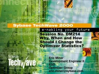
E116 Tuning the Optimizer Statistics
E116 Tuning the Optimizer Statistics. Eric Miner Senior Engineer Data Server Technology eric.miner@sybase.com. Why More On The Statistics?. Over the years I’ve received a lot of very good suggestions on how to improve presentations

E116 Tuning the Optimizer Statistics
E N D
Presentation Transcript
E116 Tuning the Optimizer Statistics • Eric Miner • Senior Engineer • Data Server Technology • eric.miner@sybase.com
Why More On The Statistics? Over the years I’ve received a lot of very good suggestions on how to improve presentations The overwhelming opinion is that you want more details via examples • “Use more examples” • “Keep questions on track” • “Use more examples” • “Give us more details” The presentation will use detailed examples of optimizer outputs to illustrate the effects of tuning the statistics
Assumptions This Is NOT going to be a ‘Basic’ Presentation We will be reviewing and discussing fairly advanced areas of Optimizer P&T, some of this you may have seen in the past. But, a little review never hurt • You’ve worked with optimizer P&T • You’re running ASE 11.9.2 or above • You understand the basics of optimization • You’ve used Traceons 302/310 and Optdiag • You’ve used the various update statistics syntax available in ASE 11.9.2 and above • You really want to know about tuning the statistics
There are Two Kinds of Optimizer Statistics • Table/Index level- describes a table and its index(es) • Page/row counts, cluster ratios, deleted and forwarded rows • Some are updated dynamically as DML occurs • page/ row counts, deleted rows, forwarded rows, cluster ratios • Stored in systabstats • Column level - describes the data to the optimizer • Histogram (distribution), density values, default selectivity values • Static, need to be updated or written directly • Stored in sysstatistics • This presentation deals with the column level statistics
Some Quick Definitions Range cell density: 0.0037264745412389 Totaldensity: 0.3208892191740000 Range selectivity: default used (0.33) In between selectivity: default used (0.25) Histogram for column: “A" Column datatype: integer Requested step count: 20 Actual step count: 10 StepWeight Value 1 0.00000000 <= 154143023 2 0.05263700 <= 154220089 3 0.05245500 <= 171522361 4 0.00000000 < 800000000 5 0.34489399 = 800000000 6 0.04968300 <= 859388217 7 0.00000000 < 860000000
Statistics On Inner Columns of Composite Indexes Stats on inner columns of composite indexes Think of a composite index as a 3D object, columns with statistics are transparent, those without statistics are opaque • Columns with statistics give the optimizer a clearer picture of an index – sometimes good, sometimes not • This is a fairly common practice • Does add maintenance • update index statistics most commonly used to do this
Statistics On Inner Columns of Composite Indexes cont. Index on columns E and B – No statistics on column b select * from TW4 where E = "yes" and b >= 959789065 and id >= 600000 and F > "May 14, 2002“ and A_A = 959000000 Beginning selection of qualifying indexes for table TW4', varno = 0, objectid 464004684. The table (Allpages) has 1000000 rows, 24098 pages, Estimated selectivity for E, selectivity = 0.527436, upper limit = 0.527436. No statistics available for B, using the default range selectivity to estimate selectivity. Estimated selectivity for B, selectivity = 0.330000.
Statistics On Inner Columns of Composite Indexes cont. The best qualifying index is ‘E_B' (indid 7) costing 49264 pages, with an estimate of 191 rows to be returned per scan of the table FINAL PLAN (total cost = 481960): varno=0 (TW4) indexid=0 () path=0xfbccc120 pathtype=sclause method=NESTED ITERATION Table: TW4 scan count 1, logical reads:(regular=24098 apf=0 total=24098) physical reads: (regular=16468 apf=0 total=16468), apf IOs used=0
Statistics On Inner Columns of Composite Indexes cont. Statistics are now on column B Estimated selectivity for E, selectivity = 0.527436, upper limit = 0.527436. Estimated selectivity for B, selectivity = 0.022199, upper limit = 0.074835. The best qualifying index is ‘E_B' (indid 7) costing 3317 pages,with an estimate of 13 rows to be returned per scan of the table FINAL PLAN (total cost = 55108): varno=0 (TW4) indexid=7 (E_B) path=0xfbd1da08 pathtype=sclause method=NESTED ITERATION Table: TW4 scan count 1, logical reads:(regular=4070 apf=0 total=4070), physical reads: (regular=820 apf=0 total=820),
Statistics On Non-Indexed Columns and Joins Stats on non-indexed columns Can’t help with index selection but can affect join ordering • Columns with statistics give the optimizer a clearer picture of the column – no hard coded assumptions have to be used • When costing joins of non-indexed columns having statistics may result in better plans than using the default values • Without statistics there will be no Total density or histogram that the optimizer can use to cost the column in the join • Yes, in some circumstances histograms can be used in costing joins – if there is a SARG on the joining column and that column is also in the join table then the SARG from the joining table can be used to filter the join table • If there is no SARG on the join column or on the joining column the Total density value (with stats) or the default value (w/o stats) will be used
Statistics On Non-Indexed Columns and Joins cont. “Inherited” SARG example select ....from TW1, TW4 where TW1.A = TW4.A and TW1.A = 10 Selecting best index for the JOIN CLAUSE: TW4.A = TW1.A TW4.A = 10 Estimated selectivity for a, selectivity = 0.003726,upper limit = 0.049683. Histogram values used select ....from TW1, TW4 where TW1.A = TW4.A and TW1.B = 10 Selecting best index for the JOIN CLAUSE: TW4.A = TW1.A Estimated selectivity for a, selectivity = 0.320889. Total density value used
Statistics On Non-Indexed Columns and Joins - Example select * from TW1,TW2 where TW1.A=TW2.A and TW1.A =805975090 A simple join with a SARG on the join column of one table Table TW2 column A has no statistics, TW1 column A does Selecting best index for the JOIN CLAUSE: (for TW2.A) TW2.A = TW1.A TW2.A = 805975090 Inherited from SARG on TW1 But, can’t help…no stats Estimated selectivity for A, selectivity = 0.100000. The best qualifying access is a table scan, costing 13384 pages, with an estimate of 50000 rows to be returned per scan of the table, using no data prefetch (size 2K I/O), in data cache 'default data cache' (cacheid 0) with MRU replacement Join selectivity is 0.100000.Inherited SARG from other table doesn’t help in this case
Statistics On Non-Indexed Columns and Joins – Example cont. Without statistics on TW2.A the plan includes a reformat with TW1 as the outer table FINAL PLAN (total cost = 2855774): varno=0 (TW1) indexid=2 (A_E_F) path=0xfbd46800 pathtype=sclause method=NESTED ITERATION varno=1 (TW2) indexid=0 () path=0xfbd0bb10 pathtype=join method=REFORMATTING • Not the best plan – but the optimizer had little to go on
Statistics On Non-Indexed Columns and Joins – Example cont. Table TW2 column A now has statistics. The inherited SARG on TW1.A can now be used to help filter the join on TW2.A Selecting best index for the JOIN CLAUSE: TW2.A = TW1.A TW2.A = 805975090 Estimated selectivity for A, selectivity = 0.001447, upper limit = 0.052948. The best qualifying access is a table scan, costing 13384 pages, with an estimate of 724 rows to be returned per scan of the table, using no data prefetch (size 2K I/O), in data cache 'default data cache' (cacheid 0) with MRU replacement Join selectivity is 0.001447.
Statistics On Non-Indexed Columns and Joins – Example cont. With statistics on TW2.A reformatting is not used and the join order has changed FINAL PLAN (total cost = 1252148): varno=1 (TW2) indexid=0 () path=0xfbd0b800 pathtype=sclause method=NESTED ITERATION varno=0 (TW1) indexid=2 (A_E_F) path=0xfbd46800 pathtype=sclause method=NESTED ITERATION
The Effects of Changing the Number of Steps (Cells) The Number of Cells (steps) Affects SARG Costing – As the Number Of Steps Changes Costing Does Too Cell weights and Range cell density are used in costing SARGs • Cell weight is used as column’s ‘upper limit’ Range cell density is used as ‘selectivity’ for Equi-SARGs – as seen in 302 output • Result(s) of interpolation is used as column ‘selectivity’ for Range SARGs • Increasing the number of steps narrows the average cell width, thus the weight of Range cells decreases • Can also result in more Frequency count cells and thus change the Range cell density value • More cells means more granular cells
The Effects of Changing the Number of Steps (Cells) cont. Average cell width = # of rows/(# of requested steps –1) • Table has 1 million rows, requested 20 steps - • 1,000,000/19 = 52,632 rows per cell • 1,000,000/199 = 5,025 rows per cell • What does this mean? • As you increase the number of steps (cells) they become narrower – representing fewer values • We’ll see that this has an effect on how the optimizer estimates the cost of a SARG
The Effects of Changing the Number of Steps (Cells) cont. Changing the number of steps – effects on Equi-SARGs select A from TW2 where B = 842000000 With 20 cells (steps) in the histogram Range cell density: 0.0012829768785739 9 0.05263200 <= 825569337 10 0.05264200 <= 842084405 SARG value falls into cell 10 Estimated selectivity for B, selectivity = 0.001283, upper limit = 0.052642. Range cell weight of density qualifying cell
The Effects of Changing the Number of Steps (Cells) cont. With 200 cells (steps) in the histogram Range cell density: 0.0002303825911991 77 0.00507200 <= 839463989 78 0.00506000 <= 842019895 • SARG value falls into cell 78 Estimated selectivity for B, selectivity = 0.000230, upper limit = 0.005060. In this case more cells result in a lower estimated selectivity • Increasing the number of steps has decreased the average width and lowered the Range cell density and the average cell weight. • Range cell density decreased because Frequency count cells appeared in the histogram
The Effects of Changing the Number of Steps (Cells) cont. Changing the number of steps – effects on Range SARGs - select * from TW2 where B between 825570000 and 830000000 With 20 cells (steps) in the histogram Range cell density: 0.0012829768785739 9 0.05263200 <= 825569337 10 0.05264200 <= 842084405 • SARG values fall into cell 10 Estimated selectivity for B, selectivity = 0.014121, upper limit = 0.052642. • Here ‘selectivity’ is the product of interpolation, ‘upper limit’ is the weight of the qualifying cell. • Interpolation estimates how much of cell will qualify for the range SARG
The Effects of Changing the Number of Steps (Cells) cont. select * from TW2 where B between 825570000 and 830000000 With 200 cells (steps) in the histogram Range cell density: 0.0002303825911991 67 0.00505200 <= 825505843 68 0.00503000 <= 825570611 69 0.00508000 <= 825635378 70 0.00504000 <= 825690418 71 0.00506400 <= 825702450 72 0.00503200 <= 825767218 73 0.00510200 <= 825831945 74 0.00425800 <= 825833785 75 0.00598400 <= 839462921 Estimated selectivity for B, selectivity = 0.029624, upper limit = 0.034606. • The SARG values now span multiple cells • Interpolation estimates amount of cells 68 and 75 to use since not all of those two cells qualify
Effects Of Changing The Total Density Value Total Density and Joins Used to cost joins when there are no SARGs on the join column(s) • If there is a SARG on the join column of this table or if there is a SARG on the corresponding joining column of the other table use the column selectivity from the index selection phase for this table. The Total density value will not be used so there is no point changing it. • This helps ‘filter’ the join of the tables • If you do need to change the Total density value use sp_modifystats or edit and read back in an optdiag file
Effects Of Changing The Total Density Valuecont. Example - Without SARG on the join or a corresponding joining column The Total density of TW4.A must be used select * from TW1,TW4 where TW1.A = TW4.A and TW1.B = 154220089 Statistics for column: “A" Range cell density: 0.0037264745412389 Total density: 0.3208892191740000
Effects Of Changing The Total Density Valuecont. Total density of TW4.A is used as the column and join selectivity Selecting best index for the JOIN CLAUSE: TW4.A = TW1.A Estimated selectivity for A, selectivity = 0.320889. costing 8670 pages, with an estimate of 320889 rows Join selectivity is 0.320889.
Effects Of Changing The Total Density Valuecont. FINAL PLAN (total cost = 9842036): varno=1 (TW4) indexid=0 () path=0xfbc8a000 pathtype=sclause method=NESTED ITERATION varno=0 (TW1) indexid=2 (A_E_F) path=0xfbc8a2e0 pathtype=join method=REFORMATTING
Effects Of Changing The Total Density Valuecont. Table: TW1 scan count 1, logical reads: (regular=11 apf=0 total=11), Physical reads: (regular=11 apf=0 total=11), Table: TW4 scan count 1, logical reads: (regular=21421 apf=0 total=21421), physical reads: (regular=3616 apf=17805 total=21421), Table: Worktable1 scan count 1000000, logical reads: (regular=2000027 apf=0 total=2000027), physical reads: (regular=0 apf=0 total=0), Total writes for this command: 17 (43 rows affected)
Effects Of Changing The Total Density Valuecont. Now change the Total density with sp_modifystats Multiply by a factor of .01 (add two zero’s) sp_modifystats testdb..TW4",“A", MODIFY_DENSITY,total,factor,".01“ Densities updated for table testdb..TW4 A Density Type Original Value New Value total 0.32088922 0.00320889
Effects Of Changing The Total Density Valuecont. With the Total density value changed Selecting best index for the JOIN CLAUSE: TW4.A = TW1.A Statistics for this column have been edited. Estimated selectivity for A, selectivity = 0.003209. costing 89 pages, with an estimate of 3209 rows Join selectivity is 0.003209.
Effects Of Changing The Total Density Valuecont. No reformatting is used and the join order is reversed FINAL PLAN (total cost = 779478): varno=0 (TW1) indexid=5 (B_F_E) path=0xfbd08800 pathtype=sclause method=NESTED ITERATION varno=1 (TW4) indexid=2 (A_nc) path=0xfbc8f800 pathtype=join method=NESTED ITERATION
Effects Of Changing The Total Density Valuecont. Table: TW1 scan count 1, logical reads: (regular=11 apf=0 total=11), Physical reads: (regular=11 apf=0 total=11), Table: TW4 scan count 9, logical reads: (regular=32 apf=0 total=32), Physical reads: (regular=9 apf=0 total=9), Total writes for this command: 0 (43 rows affected)
Adding Boundary Values To The Histogram Changing the boundary values can keep SARG values within the histogram Avoids ‘out of bounds’ costing • Out of bounds costing usually happens on an atomic column whose histogram is out of date in relation the SARG value(s) • Optimizer has only two choices for selectivity – 1 or 0 depending on the SARG operator and which end of the histogram the SARG value falls outside of
Adding Boundary Values To The Histogram cont. Histogram for column: “F" Column datatype: datetimn Requested step count: 20 Actual step count: 20 Step Weight Value 1 0.28396901 < "May 1 2002 12:00:00:000AM" 2 0.04839900 = "May 1 2002 12:00:00:000AM“ <edited> 20 0.00432500 <="May 16 2002 12:00:00:000AM“ • Since cell 1 has a weight there are NULLs in this column. In this case a little over 38% NULL
Adding Boundary Values To The Histogram cont. Out of bounds costing that uses a 0.00 selectivity select count(*) from TW1 where F = "April 30, 2002“ <= "April 30, 2002" < "May 1, 2002“ >= “May 17, 2002“ Estimated selectivity for F, selectivity = 0.000000, upper limit = 0.283969. Equi-SARG search value 'Apr 30 2002 12:00:00:000AM' is less than the smallest value in sysstatistics for this column. Estimating selectivity of index ‘ind_F', indid 6 scan selectivity 0.000000,filter selectivity 0.000000 Search argument selectivity is 0.000001. We add the 1 to the far right of the decimal to avoid divide by 0 issues later on in costing
Adding Boundary Values To The Histogram cont. Out of bounds costing that uses a 1.00 selectivity select count(*) from TW1 where F >= “Apr 30 2002” > “Apr 30 2002” <= “May 17 2002” > “May 16 2002” Estimated selectivity for F, selectivity = 1.000000. Lower bound search value 'Apr 30 2002 12:00:00:000AM' is less than the smallest value in sysstatistics for this column. Estimating selectivity of index ‘ind_F', indid 6 scan selectivity 1.000000,filter selectivity 1.000000 Search argument selectivity is 1.000000.
Adding Boundary Values To The Histogram cont. What to do if out of bounds costing is a problem Not always a problem, particularly when a selectivity of 0.000000 is used • There are two ways to deal with it • Add a dummy row to the table with a column value that allows the SARG value(s) to fall within the histogram – not always allowed • If you do add a dummy row keep in mind that it will affect the histograms of other columns. Be careful with the values you use • Write a new histogram boundary using optdiag. Edit the file and read it back in. This won’t directly affect the data, but it will extend the histogram to include the SARG values(s)
Removing Statistics Can Effect Query Plans Sometimes no statistics are better then having them This will usually be an issue when very dense columns are involved Histogram for column: “E" Step Weight Value 1 0.00000000 < "no" 2 0.47256401 = "no" 3 0.00000000 < "yes" 4 0.52743602 = "yes“ This can also show up when you have ‘spikes’ (Frequency count cells) in the distribution
Removing Statistics Can Effect Query Plans cont. select count(*) from TW4 where E = “yes” and C = 825765940 The table…has 1000000 rows, 24098 pages, Estimated selectivity for E, selectivity = 0.527436, upper limit = 0.527436. Estimating selectivity of index ‘E_AA_B', indid 6 scan selectivity 0.52743602,filter selectivity 0.527436 527436 rows, 174107 pages The best qualifying index is ‘E_AA_B' (indid 6) costing 174107 pages, with an estimate of 526 rows FROM TABLE TW4 Nested iteration. Table Scan.
Removing Statistics Can Effect Query Plans cont. delete statistics TW4(E) Estimated selectivity for E, selectivity = 0.100000. Estimating selectivity of index ‘E_AA_B', indid 6 scan selectivity 0.100000,filter selectivity 0.100000 100000 rows, 20584 pages The best qualifying index is ‘E_AA_B (indid 6) costing 20584 pages, with an estimate of 92 rows FROM TABLE TW4 Nested iteration. Index : E_AA_B Forward scan. Positioning by key.
Maintaining Tuned Statistics Tuned statistics will add to your maintenance Any statistical value you write to sysstatistics either via optdiag or sp_modifystats will be overwritten by update statistics • Keep optdiag input files for reuse • If needed get an optdiag output file, edit it and read it in • Keep scripts that run sp_modifystats • Rewrite tuned statistics after running update statistics that affects the column with the modified statistics
Monitoring Table/Index Level Fragmentation Using The Statistics Can Be Both An Optimizer and Space Management Concern The more fragmentation the less efficient page reads are • Deleted rows – fewer rows per page, affects costing • Forwarded rows – 2 I/O each, optimizer adds to costing • Empty data/leaf pages – more reads may be necessary • Clustering can get worse • Watch the DPCR of the table or APL clustered index • In general the Cluster Ratios are not a good indicator of fragmentation since they are often normally low • Use optdiag outputs to monitor these values
Monitoring Table/Index Level Fragmentation Using The Statistics cont. • ASE 12.0 and above check the ‘Space utilization’ value • ‘Large I/O efficiency’ is another value to watch Empty data page count: 0 Forwarded row count: 0.0000000000000000 Deleted row count: 0.0000000000000000 Derived statistics: Data page cluster ratio: 0.9994653835872761 Space utilization: 0.9403543288085808 Large I/O efficiency: 1.0000000000000000 • ‘Space utilization’ and ‘Large I/O efficiency’ are not used by the optimizer • The further from 1 the more fragmentation there is
The Sybase Customer newsgroups http://support.sybase.com/newsgroups The Sybase list server SYBASE-L@LISTSERV.UCSB.EDU The external Sybase FAQ http://www.isug.com/Sybase_FAQ/ Join the ISUG, ISUG Technical Journal, feature requests http://www.isug.com Where To Get More Information
The latest Performance and Tuning Guide Don’t be put off by the ASE 12.0 in the title, it covers the 11.9.2 features/functionality too http://sybooks.sybase.com/onlinebooks/group-as/asg1200e Any “What’s New” docs for a new ASE release Tech Docs at Sybase Support http://techinfo.sybase.com/css/techinfo.nsf/Home Upgrade/Migration help page http://www.sybase.com/support/techdocs/migration Where To Get More Information
Sybase Developer Network (SDN) Additional Resources for Developers/DBAs • Single point of access to developer software, services, and up-to-date technical information: • White papers and documentation • Collaboration with other developers and Sybase engineers • Code samples and beta programs • Technical recordings • Free software • Join today: www.sybase.com/developer or visit SDN at TechWave’s Technology Boardwalk