LHCb B Field Map
280 likes | 469 Vues
Monday Semin ar. IT Survey. LHCb B Field Map. Géraldine Conti. EPFL, the 21 th of May 2007. Parameterized LHCb B Field Map. Reminder of the Goal. MC Parameterization. Iterative Polynomial Fitting Method. One-go 3D Fitting Method. Choice of Regions.

LHCb B Field Map
E N D
Presentation Transcript
Monday Seminar IT Survey LHCb B Field Map Géraldine Conti EPFL, the 21th of May 2007
Reminder of the Goal MC Parameterization Iterative Polynomial Fitting Method One-go 3D Fitting Method Choice of Regions Results in the Acceptance Region Residual Parameterization Measurement Matching Method Preliminary Results Analytical Field Service May 21, 2007 Géraldine Conti Monday Seminar, EPFL Outline … Analytic Parameterization
May 21, 2007 Géraldine Conti Monday Seminar, EPFL B measurement Campaign (Dec. 2005) B Measurements done… by 3D Hall probes arranged in a fixed configuration on a movable support (fine grid of 8x8x10 cm) cover most of LHCb acceptance: Upstream : x = [-1.0, 1.0] m y = [-0.4, 0.4] m Magnet : x = [-2.7, 2.4] m y = [-1.0, 1.0] m Downstream : x = [-2.5, 2.5] m y = [-1.7, 1.7] m obtained for the two polarities (with demagnetization cycle)
May 21, 2007 Géraldine Conti Monday Seminar, EPFL Reminder of the Goal Provide an accurate determination of the B field map as close as possible to the measurements Goal What is available to perform the parameterizations? 1) TOSCA simulated B field map (grid of 10x10x10 cm) 2) Measurements (They don’t cover all the acceptance) Why is a parameterized B field map needed ? 1) The real measurements can be compared with MC data to model the residuals : Residual parameterization. 2) The extrapolation of the Residual parameterization can be realized for the regions where no measurement is available.
B-Field Map based on MC data (MC Parameterization)
Pol(4) May 21, 2007 Géraldine Conti Monday Seminar, EPFL Iterative Multipolynomial Fitting Method (1) Principle of the Method (eg. By component) : Fit By as a function of y with x,z fixed. Fit Ai as a function of z with x fixed. Fit Bj as a function of x. By(y) for x=10cm and z=830cm Ai(z) for x=210cm : Bj(x) for A0 : A0 B0 Pol(4) z x B1 A1 z x A2 B2 z x A3 B3 z x A4 B4 z x N coefficients Ai for each slice. M coefficients Bj for each slice. P coefficients Ck. At the end: N·M·P coefficients to cover the map.
Downstream region is… Magnet region… Residuals ∆(BMC - Banalytic) at z=830cm Bx(y) for x=90cm and z=[350,680] cm …reasonably described. The method works well, but not easy to achieve the final precision because of the …needs Fourier parameterization due to oscillatory pattern. difficulty of optimizing iteratively. May 21, 2007 Géraldine Conti Monday Seminar, EPFL Iterative Multipolynomial Fitting Method (2)
Fn Wn Fn Wn May 21, 2007 Géraldine Conti Monday Seminar, EPFL One-go 3D Fitting Method (1) Least square procedure : Determine the cn coefficients and the Fn functions, such that : is minimal, with Modified Gram-Schmidt orthogonalisation algorithm to keep the functions Fn that significantly reduce S : Fn are not orthogonal between them. Basis change to have Wn functions which are orthogonal between them. To decide if the Nth function is to be kept, the projection of Fn on Wn is measured and should be greater than a given value to contribute significantly to the reduction of S (the angle should be greater than a given value) . See H. Wind, Yellow report, vol.72-21,CERN,1972 ; H. Wind, Yellow report EP/81-12,CERN,1981
May 21, 2007 Géraldine Conti Monday Seminar, EPFL Implementation of the method (2) An implementation of the method is available in ROOT (TMultiDimFit Class). Some technical problems have been encountered, but solved thanks to René Brun. Configuration of the optimization : Type of Polynomials : Monomials, Legendre, Chebyshev B) Relative error accepted : C) Main limits to the number of terms in the parameterization : • Max. of terms in the final parameterization • Max. of powers for each variable x,y,z to be considered • Min. angle
May 21, 2007 Géraldine Conti Monday Seminar, EPFL Regions Definition for the B field Maps (1) Compromise between relative precision, small number of regions, small number of terms in the parameterization. Regions definitions as simple as possible. Lots of different cuttings tested : acceptance angles z coordinate x and y coordinates Cuttings with respect to B field gradient have been tested too, but the geometry of the cuttings was too complicate.
y(m) Upstream Magnet Downstream 4m z(m) 1 1.5 2 2.4 4.7 4.1 5.1 6.1 6.7 7.3 8.5 9 - 0.5m 3m 8m 10m May 21, 2007 Géraldine Conti Monday Seminar, EPFL Regions Definition for the B field Maps (2) Cutting depends mainly on only one variable (z) The same cutting is chosen for Bx,By and Bz components.
May 21, 2007 Géraldine Conti Monday Seminar, EPFL Regions Definition for the B field Maps (3) However, in the magnet region, [ymax-30cm,ymax] values have been fitted separately, but with the same z cuts to improve the fits. Bx for x=1.3m and z=4.8m By for x=1.3m and z=4.8m MC Parameterizations involve 50 to 150 terms, depending on the B field fluctuations.
TOSCA simulated By MC parameterized By May 21, 2007 Géraldine Conti Monday Seminar, EPFL By map Result (x=0m, y=0m) (1) Very good matching !
May 21, 2007 Géraldine Conti Monday Seminar, EPFL By map Result : Relative Precision (2) Relative precision : Upstream Magnet Downstream Relative precision on By < 0.001 inside the three regions
TOSCA simulated By MC parameterized By May 21, 2007 Géraldine Conti Monday Seminar, EPFL Bx map Result (x=0.4m, y=0.4m)
TOSCA simulated By MC parameterized By May 21, 2007 Géraldine Conti Monday Seminar, EPFL Bz map Result (x=0.4m, y=0.4m)
May 21, 2007 Géraldine Conti Monday Seminar, EPFL Continuity at the region boundaries Relative Discrepancy : By boundary at z=610cm Discrepancy between the two By parameterizations at the z=610cm boundary Discrepancy between By parameterizations at the 14 boundaries The relative discrepancy between MC parameterizations at the boundary of two regions is in the same order of the fit precision (~10-3).
May 21, 2007 Géraldine Conti Monday Seminar, EPFL Out of acceptance regions Parameterization needed, but with a less acurate precision. The Downstream region has been already parameterized. Problems (peaks) are encountered for the Upstream and Magnet regions to find a good parameterization, because we are inside material. Upstream Magnet Downstream
Matching with the measurements (Residual Parameterization)
May 21, 2007 Géraldine Conti Monday Seminar, EPFL Clean-up of the measurements Some non-physical behaviours observed in the measurements, which can perturb the parameterizations. Clean-up of the measurements done in the three regions (started by Adlene Hicheur). Clean-up
May 21, 2007 Géraldine Conti Monday Seminar, EPFL Matching Method Calculate the B values with the MC Parameterizations at the same measurement coordinates (x,y,z). Measurements Analytic values Residuals Parameterize the residuals (Bmeasurements - Banalytic values) : Analytic Parameterization = MC Parameterization + Residual Parameterization Extrapolate the Residual Parameterization to regions where no measurement is available.
x=4cm, y=4cm, Upstream x=4cm, y=4cm, Magnet Interpolation MC Parameterization Measurements Analytic Parameterization (MC + Residual Parameterization) May 21, 2007 Géraldine Conti Monday Seminar, EPFL By Residual Results (1) Non negligible corrections for the most important B component (By) near the centre (x~0cm and y~cm) !
x=100cm, y=4cm, Magnet x=204cm, y=164cm x=140cm, y=140cm Interpolation MC Parameterization Measurements Analytic Parameterization (MC + Residual Parameterization) May 21, 2007 Géraldine Conti Monday Seminar, EPFL By Residual Results (2) The most important discrepancies between MC data and measurements are found for big x and/or y values
May 21, 2007 Géraldine Conti Monday Seminar, EPFL Reverse Polarisation By Residuals (3) x=100cm, y=4cm, Magnet Interpolation MC Parameterization -(Reverse Polarisation Measurements) Analytic Parameterization (MC + Residual Parameterization) The values obtained with the Analytic Parameterization (found for positive polarisation measurements) seems to match well with the reverse polarisation measurements. More comparisons still have to be done…
Only the Residual Parameterization could be used with the interpolation method to give more accurate B values . A new file with B values used by the interpolation could be generated with the help of the Analytic Parameterization . May 21, 2007 Géraldine Conti Monday Seminar, EPFL Analytic Field Service It has been implemented in Det/Magnet, but is not available in CVS yet. However, according to preliminary tests, the speed of the B value access seems to be an issue… Speed tests forseen with tracks Several scenarios : 1) Analytic Parameterization is faster or of the order of time of the interpolation method : Best scenario : faster access and more accurate B values . 2) Analytic Parameterization is slower than the interpolation :
May 21, 2007 Géraldine Conti Monday Seminar, EPFL Conclusions and Perspectives Parameterization based on MC simulation data has been succesfully performed in the acceptance region by the One-go 3D Fitting Method and reaches a rel. Prec. < 10-3 for the By component in all the 3 regions. Parameterization of the By residuals gives the expected more accurate B values with respect to the measurements. On-going / to do : MC parameterization of the « Out of acceptance » Magnet and Upstream regions. Residual parameterizations for Bx and Bz. Extrapolate the Residual parameterizations to regions where no measurements are available. Speed tests of the Analytic Service with tracks.