Download
1 / 38
380 likes | 544 Vues
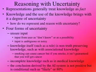
Reasoning with Uncertainty. We briefly examined certainty factors earlier in the semester, but for the most part, we have only studied knowledge that is true/false or truth preserving but the world is full of uncertainty, we need mechanisms to reason over that uncertainty

E N D
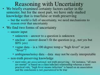
Reasoning with Uncertainty • We briefly examined certainty factors earlier in the semester, but for the most part, we have only studied knowledge that is true/false or truth preserving • but the world is full of uncertainty, we need mechanisms to reason over that uncertainty • We find two forms of uncertainty • unsure input • unknown – answer to a question is unknown • unclear – answer doesn’t fit the question (e.g., not yes but 80% yes) • vague data – is a 100 degree temp a “high fever” or just “fever”? • ambiguous/noisy data – data may not be easily interpretable • non-truth preserving knowledge • most rules are associational, not truth preserving – for instance, “all men are mortal” is based on a class/subclass relationship whereas a more practical rule, “high fever means infection” is based on an association and the conclusion is not guaranteed to be true
Monotonicity • Monotonicity – starting with a set of axioms, assume we draw certain conclusions • if we add new axioms, previous conclusions must remain true • the knowledge space can only increase, new knowledge should not rule out items previously thought to be true • example: assume that person X was murdered and through various axioms about suspects and alibis, we conclude person Y committed the murder • later, if we add new evidence, our previous conclusion that Y committed the murder must remain true • obviously, the real world doesn’t work this way (assume for instance that we find that Y has a valid alibi and Z’s alibi was a person who we discovered was lying because of extortion)
The Closed World Assumption • In monotonic reasoning, if something is not explicitly known or provable, then it is false • this assumption in our reasoning can easily lead to faulty reasoning because its impossible to know everything • How can we resolve this problem? • we must either introduce all knowledge that is required to solve the problem at the beginning of problem solving • or we need another form of reasoning aside from monotonic logic • The logic that we have explored so far (first order predicate calculus with chaining or resolution) is monotonic (so is the Prolog system) • so now we turn to non-monotonic logic
Non-monotonicity • Non-monotonic logic is a logic in which, if new axioms are introduced, previous conclusions can change • this requires that we update/modify previous proofs • this could be very computationally costly as we might have to redo some of our proofs • We can enhance our previous algorithms • in logic, add M before a clause meaning “it is consistent with” • for all X: bright(X) & student(X) & studies(X,CSC) & M good_economy(time_of_graduation) job(X, time_of_graduation) • a bright student who studies CSC will find a job at graduation if the economy is good – we may assume the CSC grad will find a job even if we don’t know about the economy – that is, we are making an assumption in the face of a missing piece of knowledge • in a production system, add unless clauses to rules • if X is bright, X is a student and X studies computer science, then X will get a job at the time of graduation unless the economy is not good at that time • These are forms of assumption-based reasoning
Dependency Directed Backtracking • To reduce the computational cost of non-monotonic logic, we need to be able to avoid re-searching the entire search space when a new piece of evidence is introduced • otherwise, we have to backtrack to the location where our assumption was introduced and start searching anew from there • In dependency directed backtracking, we move to the location of our assumption, make the change and propagate it forward from that point without necessarily having to re-search from scratch • as an example, you have scheduled a meeting on Tuesday at 12:15 because everyone indicated that they were available • but now, you cannot find a room, so you backtrack to the day and change it to Thursday, but you do not re-search for a new time because you assume if everyone was free on Tuesday, they will be free on Thursday as well
Truth Maintenance Systems • In a TMS, inferences are supported by evidence • support is directly annotated in the representation so that new evidence can be mapped to conclusions easily • if some new piece of evidence is introduced which may overturn a previous conclusion, we need to know if this violates an assumption • if so, we negate the assumption and follow through to see what conclusions are no longer true • The TMS is a graph-based representation to support dependency-directed backtracking • this simplifies how to make changes when new evidence is introduced or when an assumption is shown to be false • there are several forms of TMS, we will concentrate on the justification TMS (JTMS) but others include assumption-based TMS (ATMS), logic-based TMS (LTMS), and multiple belief reasoners (MBR)
Justification Truth Maintenance System • The JTMS is a graph implementation whereby each inference is supported by evidence • an inference is supported by items that must be true (labeled as IN items) and those that must be false (labeled as OUT items), things we assume false will be labeled OUT • when a new piece of • evidence is introduced, • we examine the pieces • of evidence to see if • this either changes it • to false or contradicts • an assumption, and • if so, we change any • inferences that were • drawn from this • evidence to false, and propagate this across the graph
The ABC Murder Mystery • As an example, we consider a murder • Some pieces of knowledge are: • a person who stands to benefit from a murder is a suspect unless the person has an alibi • a person who is an enemy of a murdered person is a suspect unless the person has an alibi • an heir stands to benefit from the death of the donor unless the donor is poor • a rival stands to benefit from the death of their rival unless the rivalry is not important • an alibi is valid if you were out of town at the time unless you have no evidence to support this • a picture counts as evidence • a signature in a hotel registry is evidence unless it is forged • a person vouching for a suspect is an alibi unless the person is a liar
ABC Murder Mystery Continued • Our suspects are • Abbott (A), an heir, Babbitt (B), a rival, Cabbott (C) an enemy • we do not know if the victim was wealthy or poor and we do not know if B’s rivalry with the victim was important or not • A claims to have been in Albany that weekend • B claims to have been with his brother-in-law • C claims to have been in the Catskills watching a ski meet • we have no evidence to back up A, B, or C’s alibis, so they are all suspects * denotes evidence directly supported by input + denotes IN evidence (must be true) – denotes OUT evidence (assumed false) Since we have no evidence of an alibi for any of A, B, C, and because each is a known heir/enemy/rival, we conclude all three are suspects
New Evidence Comes To Light • Abbott produces evidence that he was out of town • his signature is found in the hotel registry of a respectable hotel in Albany, NY • Babbitt’s brother-in-law signs an affidavit stating that Babbitt did in fact spend the weekend with him • B has an alibi (not in town) and is no longer a suspect We have an alibi for A changing the assumption to true and therefore ruling him out as a suspect Similarly for B, but there is no change made to C, so C remains a suspect
But Then… • B’s brother-in-law has a criminal record for perjury, so he is a known liar • thus, B’s alibi is not valid and B again becomes a suspect • A friend of C’s produces a photograph of C at the meet, shown with the winner • the photograph supports C’s claim that he was not in town and therefore is a valid alibi, C is no longer a suspect With these final modifications, B becomes our only suspect
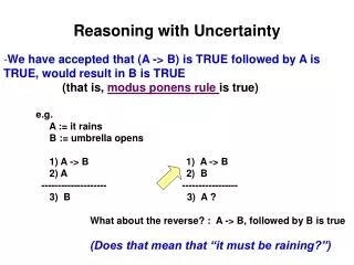
Abduction • In traditional logic, Modus Ponens tell us that if we have • A B • A • we conclude B • In abduction, we have instead • A B • B • we conclude A • The idea here is that we are saying “A can cause B”, “B happened”, we conclude “A was its cause” • this form of reasoning is useful for diagnosis (as an example) but it is not truth-preserving • consider that we know that if the battery has lost its charge then the car won’t start • if the car doesn’t start, we can conclude that the battery lost its charge • the reason this isn’t truth preserving is because there are other possible causes for the car not starting (bad starter, no fuel, etc)
How Abduction Can be Truth-Preserving • We can still use abduction, but it now takes more work: • assume there are several causes for B: • A1 B, A2 B, A3 B, A4 B • if we can rule out A1, A2 and A3 (that is, we introduce ~A1, ~A2, ~A3) then we conclude A4 • Diagnosis is commonly performed through abduction • although in the case of a medical doctor • the possible causes A1, A2, A3, A4 are not ruled out • instead the doctor assigns plausibility values (likelihoods) to each of A1, A2, A3 and A4 so that if A1, A2 and A3 are very unlikely, A4 is the best explanation • how do we get these plausibility values?
Set Covering • In diagnosis, there may be multiple contributing factors or multiple causes of the symptoms • Assume that the following malfunctions (H1-H5, which we will call our hypotheses) can cause the symptoms (observations, O1-O5) as shown • H1 O1, O2, O3 H2 O1, O4 • H3 O2, O3, O5 H4 O5 • H5 O2, O4, O5 • O1, O2 and O5 are observed, and we find H1-H5 to be all plausible (say “likely”), what is our best explanation? • {H1, H4} explains them all but includes O3 (not observed) • {H2, H5} explains them all but includes O4 (twice) (not observed) • {H1, H3} explains them all but includes O3 (twice) • {H1, H4, H5} explains them all but H4 is superfluous • Mathematically, this problem is known as set covering
Controlling Abduction • Set covering is an NP-complete problem • it is computationally expensive because it requires trying all combinations of subsets (of H’s) until we have a cover • it should be apparent that while diagnosticians use abduction, they do not resort to complete set covering, that is, they solve the problem in less amount of time • Factors involved in set covering/abduction • minimal explanation – the explanation with the fewest hypotheses • parsimonious explanation – no superfluous parts • highest rated explanation – the explanation should contain the most highly evaluated hypotheses (if we evaluate them) • these first three combined are known as cost-based abduction • consistent explanation – the explanation should not include hypotheses that contradict each other • this last one is known as coherence-based abduction
Forms of Abduction • Aside from trying to build a complete and consistent explanation without superfluous parts, we often want to select the explanation that best explains the data • this requires that we somehow gage the hypotheses in terms of their plausibilities • How? • many different approaches have been taken • structured matching • certainty factors • Bayesian probabilities • fuzzy logic • neural networks • structured matching was mentioned earlier in the semester, we will revisit it in the on-line notes, and we will hold off on looking at neural networks until chapter 11
Certainty Factors • First used in the MYCIN system, the idea is that we will attribute a measure of belief to any conclusion that we draw • CF(H | E) = MB(H | E) – MD(H | E) • certainty factor for hypothesis H given evidence E is the measure of belief we have for H minus measure of disbelief we have for H • CFs are applied to any hypothesis that we draw by combining CFs of previous hypotheses that are used in the condition portion of the given rule and the CF given to the rule itself • To use CFs, we need • to annotate every rule with a CF value • this comes from the expert • ways to combine CFs when we use AND, OR, • Combining rules are straightforward: • for AND use min: CF(X AND Y) = min(CF(X), CF(Y)) • for OR use max: CF (X OR Y) = max(CF(X), CF(Y)) • for use * (multiplication): CF(X Y) = CF(X) * CF(Y)
CF Example • Assume we have the following rules: • A B (.7) • A C (.4) • D F (.6) • B AND G E (.8) • C OR F H (.5) • We know A, D and G are true (so each have a value of 1.0) • B is .7 • A is 1.0, the rule is true at .7, so B is true at 1.0 * .7 = .7 • C is .4 (CF(A) * .4 = 1 * .4) • F is .6 (CF(D) * .6) = 1 * .6) • B AND G is min(.7, 1.0) = .7 (G is 1.0, B is .7) • E is .7 * .8 = .56 • C OR F is max(.4, .6) = .6 • H is .6 * .5 = .30
Continued • Another combining rule is needed when we can conclude the same hypothesis from two or more rules • we already used C OR F H (.5) to conclude H with a CF of .30 • let’s assume that we also have the rule E H (.5) • since E is .56, we have H at .56 * .5 = .28 • We now believe H at .30 and at .28, which is true? • the two rules both support H, so we want to draw a stronger conclusion in H since we have two independent means of support for H • We will use the formula CF1 + CF2 – CF1*CF2 • CF(H) = .30 + .28 - .30 * .28 = .496 • our belief in H has been strengthened through two different chains of logic
CF Advantages and Disadvantages • The nice aspects of CFs are that • it gives us a mechanism to evaluate hypotheses in order to select the best one(s) for our explanation • the formulas are simple to apply • experts often think in terms of plausibilities, so getting an expert to supply the CF for a given rule is straight-forward • The disadvantages are that • CFs are ad hoc (not defined through any formal algebra) • no guideline for providing CFs for rules • multiple experts may give you inconsistent CFs • a single expert may give you less consistent values over time • CFs are only provided for rules • input is always given the value of 1.0 • Many researchers liked the idea of CFs but were not encouraged by the lack of formalism, so other approaches have been developed
Fuzzy Logic • Prior to CFs, Zadeh introduced fuzzy logic (FL) as a means to represent “shades of grey” into logic • traditional logic is two-valued, true or false only • FL allows terms to take on values in the interval [0, 1] (that is, real numbers between 0 and 1) • Being a logic, Zadeh introduced the algebra to support logical operators of AND, OR, NOT, • X AND Y = min(X, Y) • X OR Y = max(X, Y) • NOT X = (1 – X) • X Y = X * Y • Where the values of X, Y are determined by where they fall in the interval [0, 1]
Fuzzy Set Theory • Fuzzy sets are to normal sets what FL is to logic • fuzzy set theory is based on fuzzy values from fuzzy logic but includes set operators (is an element of, subset, union, intersection) instead of logic operations • The basis for fuzzy sets is defining a fuzzy membership function for a set • a fuzzy set is a set of items in the set along with their membership values which denote how closely each individual item is to being in that set • Example: the set tall might be denoted as • tall = { x | f(x) = 1.0 if height(x) > 6’2”, .8 if height(x) > 6’, .6 if height(x) > 5’10”, .4 if height(x) > 5’8”, .2 if height(x) > 5’6”, 0 otherwise} • so we can say that a person is tall at .8 if they are 6’1” or we can say that the set of tall people are {Anne/.2, Bill/1.0, Chuck/.6, Fred/.8, Sue/.6}
Fuzzy Membership Function • Typically, a membership function is a continuous function (often represented in a graph form like above) • given a value y, the membership value for y is u(y), determined by tracing the curve and seeing where it falls on the u(x) axis • How do we define a membership function? • for instance, is our fuzzy set for Tall realistic? • defining membership functions remains an open question
Using Fuzzy Logic/Sets • 1. fuzzify the input(s) using fuzzy membership functions • 2. apply fuzzy logic rules to draw conclusions • we use the previous rules for AND, OR, NOT, • 3. if conclusions are supported by multiple rules, combine the conclusions • like CF, we need a combining function, this may be done by computing a “center of gravity” using calculus • 4. defuzzify conclusions to get specific conclusions • defuzzification requires translating a numeric value into an actionable item • FL is often applied to domains where we can easily derive fuzzy membership functions and require few rules • fuzzy logic begins to break down when we have more than a dozen or two rules • we visit a complete example in the on-line notes
Using Fuzzy Logic • The most common applications for FL are for controllers • devices that, based on input, make minor modifications to their settings – for instance • air conditioner controller that uses the current temperature, the desired temperature, and the number of open vents to determine how much to turn up or down the blower • camera aperture control (up/down, focus, negate a shaky hand) • a subway car for braking and acceleration • FL has been used for expert systems • but the systems tend to perform poorly when more than just a few rules are chained together • in our previous example, we just had 5 stand-alone rules • when we chain rules, the fuzzy values are multiplied (e.g., .5 from one rule * .3 from another rule * .4 from another rule, our result is .06)
Dempster-Shaefer Theory • D-S Theory goes beyond CF and FL by providing us two values to indicate the utility of a hypothesis • belief – as before, like the CF or fuzzy membership value • plausibility – adds to our belief by determining if there is any evidence (belief) for opposing the hypothesis • We want to know if h is a reasonable hypothesis • we have evidence in favor of h giving us a belief of .7 • we have no evidence against h, this would imply that the plausibility is greater than the belief • p(h) = 1 – b(~h) = 1 (since we have no evidence against h, ~h = 0) • Consider two hypotheses, h1 and h2 where we have no evidence in favor of either, so b(h1) = b(h2) = .5 • we have evidence that suggests ~h2 is less believable than ~h1 so that b(~h2) = .3 and b(~h1) = .5 • h1 = [.5, .5] and h2 = [.5, .7] so h2 is more believable • the details for D-S theory are presented in the notes
Bayesian Probabilities • Bayes derived the following formula • p(h | E) = p(E | h) * p(h) / sum for all i (p(E | hi) * p(hi)) • the probability that h is true given evidence E • p(h | E) – conditional probability • what is the probability that h is true given the evidence E • p(E | h) – evidential probability • what is the probability that evidence E will appear if h is true? • p(h) – prior probability (or a priori probability) • what is the probability that h is true in general without any evidence? • the denominator normalizes the conditional probabilities to add up to 1 • To solve a problem with Bayesian probabilities • we need to accumulate the probabilities for all hypotheses h1, h2, h3 of p(h1 | E), p(h2 | E), p(h3 | E), …, p(E | h1), p(E | h2), p(E | h3), … and p(h1), p(h2), p(h3), … and then its just a straightforward series of calculations
Example • The sidewalk is wet, we want to determine the most likely cause • it rained overnight (h1) • we ran the sprinkler overnight (h2) • wet sidewalk (E) • Assume the following • there was a 50% chance of rain – p(h1) = .5 • sprinkler is run two nights a week – p(h2) = 2/7 = .28 • p(wet sidewalk | rain overnight) = .8 • p(wet sidewalk | sprinkler) = .9 • Now we compute the two conditional probabilities • p(h1 | E) = (.5 * .8) / (.5 * .8 + .28 * .9) = .61 • p(h2 | E) = (.28 * .9) / (.5 * .8 + .28 * .9) = .39
Independent Events • There is a flaw with our previous example • if it is likely that it will rain, we will probably not run the sprinkler even if it is the night we usually run it, and if it does not rain, we will probably be more likely to run the sprinkler the next night • So we have to be aware of whether events are independent or not • two events are independent if P(A & B) = P(A) * P(B) • where & means “intersect” • when P(B) <> 0, then P(A) = P(A | B) • knowing B is true does not affect the probability of A being true • We can also modify our computation by using the formula for conditional independent events • P(A & B | C) = P(A | C) * P(B | C) • again, & is used to mean intersection • we will expand on this shortly
Multiple Pieces of Evidence • In our wet sidewalk example, E consisted of one piece of evidence, wet sidewalk • what if we have many pieces of evidence? • Consider a diagnostic case where there are 10 possible symptoms that we might look for to determine whether a patient has a cold (h1), flu (h2) or sinus infection (h3) • E is some subset of {e1, e2, e3, e4, e5, e6, e7, e8, e9, e10} • To use Bayes’ formula, we need to know • p(h1), p(h2), p(h3) as well as • p(e1 | h1), p(e1 | h2), p(e1 | h3) • p(e2 | h1), p(e2 | h2), p(e2 | h3) • p(e3 | h1), p(e3 | h2), p(e3 | h3) • …
Continued • But our patient may have several symptoms • So we also need • p(e1, e2 | h1), p(e1, e2 | h2), p(e1, e2 | h3) • p(e1, e3 | h1), p(e1, e3 | h2), p(e1, e3 | h3) • p(e2, e3 | h1), p(e2, e3 | h2), p(e2, e3 | h3) • p(e1, e2, e3 | h1), p(e1, e2, e3 | h2), p(e1, e2, e3 | h3) • How many different probabilities will we need? • with 10 pieces of evidence, there are 210 = 1024 different combinations for E, so we will need 3 * 1024 = 3072 evidential probabilities (to go along with the 3 prior probabilities, one for each hypothesis) • imagine if E comprised a set of 50 pieces of evidence instead!
Advantages and Disadvantages • There two appealing features of probabilities • the approach is formal (unlike CFs and unlike the creation of fuzzy membership functions, which are ad hoc) • probabilities are easy to compile through statistics • p(flu) = number of people who had the flu this year / number of people in the pool • p(fever | flu) = number of people with the flu who had a fever / number of people in the pool • The primary disadvantages are • the need for a great number of probabilities • probabilities can be biased • for instance, is p(flu) accurate if we gather the data in the summer time rather than in the winter? • the awkwardness if events are not independent (an example is in the notes for you to read on-line)
Bayesian Net • We can apply the Bayesian formulas for independent and conditionally dependent events in a network form • we want to determine the likely cause for seeing orange barrels, flashing lights and bad traffic on the highway • two hypotheses: construction, accident (see the figure below) • notice T (bad traffic) can be caused by either construction or an accident, orange barrels are only evidence of construction and flashing lights are only evidence of an accident (although it could also be that a driver has been pulled over) • construction and accident are not directly related to each other – this will help simplify the problem
Computing the Cause • We want to compute the cause: construction or accident? • first we derive a chain rule to compute a chain of probabilities to handle the dependencies as shown in the figure • p(a, b) = p(a | b) * p(b) – that is, the probability of both a & b happening is computed as p(a | b) * p(b) • Extending this further, we have p(a, b, c) = p(a) * p(b | a) * p(c | a, b) • Returning to our Bayesian network, p(C, A, B, T, L) = p(C) * p(A | C) * p(B | C, A) * p(T | B, C, A, B) * p(L | C, A, B, T) • with 5 events/conditions, we need 25 = 32 probabilities • We can reduce p(C, A, B, T, L) to p(C) * p(A) * p(B | C) * p(T | C, A) * p(L, A) • because C and A are not linked, p(A | C) = p(A), p(B | C, A) = p(B | C) • thus we reduce the total number of terms from 32 to 20 • we will visit an example from the book in the on-line notes
Markov Models • Like the dynamic Bayesian network, a Markov model is a graph composed of • states that represent the state of a process • edges that indicate how to move from one state to another where edge is annotated with a probability indicating the likelihood of taking that transition • An ordinary Markov model contains states that are observable so that the transition probabilities are the only mechanism that determines the state transitions • a hidden Markov model (HMM) is a Markov model where the probabilities are actually probabilistic functions that are based in part on the current state, which is hidden (unknown or unobservable) • determining which transition to take will require additional knowledge than merely the state transition probabilities
A Markov Model • In the Markov model, we move from state to state based on simple probabilities • going from S3 to S2 has a likelihood of a32 • going from S3 to S3 has a likelihood of a33 • likelihoods are usually computed stochastically (statistically) • Sequences of probabilities are multiplied together, for instance probability of 3 sunny days in a row is .8 * .8 (assume the first day is sunny)
HMM • Most problems cannot be solved by a Markov model because there are unknown states • in speech recognition, we can build a Markov model to predict the next word in an utterance by using the probabilities of how often any given word follows another • how often does “lamb” follow “little”? • But in speech recognition, there is intention here • we do not know what the speaker is intending to say, but we must identify it, so, we add to our model hidden (unobservable) states and appropriate probabilities for transitions • the observable states are the elements of the acoustic signal, that is, things we can analyze • and the hidden states are the elements of the utterance (e.g., phonemes), we must search the HMM to determine what hidden state best represents the input utterance
Example HMM • Here, X1, X2 and X3 are the hidden states • y1, y2, y3, y4 are observations • Aij are the transition probabilities of moving from state i to state j • bij make up the output probabilities from hidden node i to observation j – that is, what is the probability of seeing output yj given that we are in state xi? • Three problems associated with HMMs • Given HMM and output sequence, compute most likely state transitions • Given HMM, compute the probability of a given output sequence • Given HMM and output sequence, compute the transition probabilities • See the notes for more details