Basic Optimization Theory
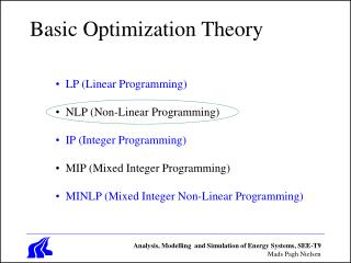
Basic Optimization Theory. LP (Linear Programming) NLP (Non-Linear Programming) IP (Integer Programming) MIP (Mixed Integer Programming) MINLP (Mixed Integer Non-Linear Programming). Types Of Optimization. Parameter Optimization Configuration Optimization

Basic Optimization Theory
E N D
Presentation Transcript
Basic Optimization Theory • LP (Linear Programming) • NLP (Non-Linear Programming) • IP (Integer Programming) • MIP (Mixed Integer Programming) • MINLP (Mixed Integer Non-Linear Programming) Analysis, Modelling and Simulation of Energy Systems, SEE-T9 Mads Pagh Nielsen
Types Of Optimization • Parameter Optimization • Configuration Optimization • Operational Optimization • Topology Optimization Analysis, Modelling and Simulation of Energy Systems, SEE-T9 Mads Pagh Nielsen
Topology Optimization Analysis, Modelling and Simulation of Energy Systems, SEE-T9 Mads Pagh Nielsen
max. min. f x x x or ( , ,..., ) 1 2 n subject to: g x x x b £ ( , ,..., ) 1 1 2 1 n g x x x b £ ( , ,..., ) 2 1 2 2 n L L g x x x b £ ( , ,..., ) m 1 2 m n The General Non-Linear Problem Objective Function Constraints Design Space Analysis, Modelling and Simulation of Energy Systems, SEE-T9 Mads Pagh Nielsen
Extrema: Ordering Situation $ 1000 800 Total Cost 600 400 Transport Cost Ordering Cost 200 OPT. 0 0 10 20 30 40 50 Order Quantity Analysis, Modelling and Simulation of Energy Systems, SEE-T9 Mads Pagh Nielsen
Extrema: Heat Exchanger $ 1000 800 Total Cost 600 400 Material Cost Energy Cost 200 OPT. 0 0 100 200 300 400 500 Heat Exchanger Area Analysis, Modelling and Simulation of Energy Systems, SEE-T9 Mads Pagh Nielsen
global max stationary point f(x) local max local min local min x Local vs. Global Extrema Analysis, Modelling and Simulation of Energy Systems, SEE-T9 Mads Pagh Nielsen
Convexity f(x) f(x) Concave Function Convex Function f(x2) f(x1)+(1- )f(x2) f(x1) f(x1 +(1- )x2) x1 x2 x1+(1-)x2 x x f(x) is a convex function if and only if for any given two points x1 and x2 in the function domain and for any constant 0 1 f(x1 +(1- )x2) f(x1)+(1- )f(x2) Analysis, Modelling and Simulation of Energy Systems, SEE-T9 Mads Pagh Nielsen
The Hessian • The gradient vector of f at x • The Hessian Matrix of f at x Analysis, Modelling and Simulation of Energy Systems, SEE-T9 Mads Pagh Nielsen
Conditions for convexity How can we use Hessian to determine whether or not f(x) is convex? • H(x) is positive semi-definite if and only if xTHx≥ 0 for all x and there exists and x 0 such that xTHx = 0. => Convexity • H(x) is positive definite if and only if xTHx> 0 for all x0. • H(x) is indefinite if and only if xTHx> 0 for some x, and xTHx< 0 for some other x. Analysis, Modelling and Simulation of Energy Systems, SEE-T9 Mads Pagh Nielsen
objective function level curve objective function level curve optimal solution optimal solution Feasible Region Feasible Region nonlinear objective, linear constraints linear objective, nonlinear constraints objective function level curve objective function level curves optimal solution optimal solution Feasible Region Feasible Region nonlinear objective, nonlinear constraints nonlinear objective, linear constraints Possible Solutions To Convex Problems Analysis, Modelling and Simulation of Energy Systems, SEE-T9 Mads Pagh Nielsen
Line Search Line search techniques are in essence optimization algorithms for one dimensional minimization problems. They are often regarded as the backbones of nonlinear optimization algorithms. Typically, these techniques search a bracketed interval. Often, unimodality is assumed. x* a b Exhaustive search requires N = (b-a)/ + 1 calculations to search the above interval, where is the resolution. Analysis, Modelling and Simulation of Energy Systems, SEE-T9 Mads Pagh Nielsen
Bracketing Algorithm x2 a x1 b Two point search (dichotomous search) for finding the solution to minimizing ƒ(x): 0) assume an interval [a,b] 1) Find x1 = a + (b-a)/2 - /2 and x2 = a+(b-a)/2 + /2 where is the resolution. 2) Compare ƒ(x1) and ƒ(x2) 3) If ƒ(x1) < ƒ(x2) then eliminate x > x2 and set b = x2 If ƒ(x1) > ƒ(x2) then eliminate x < x1 and set a = x1 If ƒ(x1) = ƒ(x2) then pick another pair of points 4) Continue placing point pairs until interval < 2 Analysis, Modelling and Simulation of Energy Systems, SEE-T9 Mads Pagh Nielsen
Golden Section Search b a Discard a - b a b In Golden Section, you try to have b/(a-b) = a/b which implies b*b = a*a - ab Solving this gives a = (b ± b* sqrt(5)) / 2 a/b = -0.618 or 1.618 (Golden Section ratio) Note that 1/1.618 = 0.618 Analysis, Modelling and Simulation of Energy Systems, SEE-T9 Mads Pagh Nielsen
Golden Section Search Algorithm {Initialize} x1 = a + (b-a)*0.382 x2 = a + (b-a)*0.618 f1 = ƒ(x1) f2 = ƒ(x2) {Loop} if f1 > f2 then a = x1; x1 = x2; f1 = f2 x2 = a + (b-a)*0.618 f2 = ƒ(x2) else b = x2; x2 = x1; f2 = f1 x1 = a + (b-a)*0.382 f1 = ƒ(x1) end x2 a x1 b Analysis, Modelling and Simulation of Energy Systems, SEE-T9 Mads Pagh Nielsen
X2 Local optimal solution C Local and global optimal solution F E Feasible Region G B A D X1 The 2D case Analysis, Modelling and Simulation of Energy Systems, SEE-T9 Mads Pagh Nielsen
The 2D case (From John Rasmussen, 1999) Analysis, Modelling and Simulation of Energy Systems, SEE-T9 Mads Pagh Nielsen
Example: Heat Exchanger Problem: Find the radius of tubes in a heat exchanger to maximize the total surface area. (The magnitude of pressure drops are not considered) Analysis, Modelling and Simulation of Energy Systems, SEE-T9 Mads Pagh Nielsen
Setting up the problem: What is the best value of r ? What if we added a maximum allowable pressure drop? Analysis, Modelling and Simulation of Energy Systems, SEE-T9 Mads Pagh Nielsen
3 T 2 1 4 s Ideal Rankine Cycle Balance • Assumptions: steady flow process, no generation, neglect KE and PE changes for all four devices, • First Law: 0 = (net heat transfer in) - (net work out) + (net energy flow in) • 0 = (qin - qout) - (Wout - Win) + (hin - hout) • 1-2: Pump (q=0) • Wpump = h2 - h1 = v(P2-P1) • 2-3: Boiler (W=0) qin = h3 - h2 • 3-4: Turbine (q=0) Wout = h3 - h4 • 4-1: Condenser (W=0) qout = h4 - h1 Thermal efficiencyh = Wnet/qin = 1 - qout/qin = 1 - (h4-h1)/(h3-h2) Wnet = Wout - Win = (h3-h4) - (h2-h1) Analysis, Modelling and Simulation of Energy Systems, SEE-T9 Mads Pagh Nielsen
3 T 2 T 1 4 2 s 1 s Thermal efficiency can be improved by manipulating the temperatures and/or pressures in various components(a) Lowering the condensing pressure (lowers TL, but decreases quality, x4)(b) Superheating the steam to a higher temperature (increases TH but requires higher temp materials)(c) Increasing the boiler pressure (increases TH but requires higher temp/press materials) Possibility for improvement of thermal efficiency: T (c) increase pressure 3 (b) Superheating 2 1 2 4 4 1 s Low quality high moisture content (a) lower pressure(temp) Red area = increase in W net Blue area = decrease in W net Analysis, Modelling and Simulation of Energy Systems, SEE-T9 Mads Pagh Nielsen
Reheating • The optimal way of increasing the boiler pressure without increasing the moisture content in the exiting vapor is to reheat the vapor after it exits from a first-stage turbine and redirect this reheated vapor into a second turbine. 3 T high-P turbine 5 high-P turbine Low-P turbine 3 low-P turbine boiler 4 4 4 5 6 2 1 2 pump 6 1 condenser s Analysis, Modelling and Simulation of Energy Systems, SEE-T9 Mads Pagh Nielsen
Reheating • Reheating allows one to increase the boiler pressure without increasing the moisture content in the vapor exiting from the turbine. • By reheating, the average temperature of the vapor entering the turbine is increased, thus, it increases the thermal efficiency of the cycle. • Multistage reheating is possible but not practical. One major reason is because the vapor exiting will be superheated vapor at higher temperature, thus, decrease the thermal efficiency. • Energy analysis: Heat transfer and work output both change • qin = qprimary + qreheat = (h3-h2) + (h5-h4) • Wout = Wturbine1 + Wturbine2 = (h3-h4) + (h5-h6) Analysis, Modelling and Simulation of Energy Systems, SEE-T9 Mads Pagh Nielsen
Regeneration • From 2-2’, the average temperature is very low, therefore, the heat addition process is at a lower temperature and therefore, the thermal efficiency is lower. • Use a regenerator to heat the liquid (feedwater) leaving the pump before sending it to the boiler. This increases the average temperature during heat addition in the boiler, hence it increases efficiency. higher temp heat addition Lower temp heat addition 5 3 T T 2’ 4 6 2 3 2 7 1 4 1 s s Use regenerator to heat up the feedwater Analysis, Modelling and Simulation of Energy Systems, SEE-T9 Mads Pagh Nielsen
Regeneration Cycle • Improve efficiency by increasing feedwater temperature before it enters the boiler. • Two Options: • Open feedwater : Mix steam with the feedwater in a mixing chamber. • Closed feedwater: No mixing. Open FWH 5 T 5 4 (y) 6 6 Open FWH 7 boiler (y) (1-y) 2 (1-y) 3 3 2 4 Pump 2 7 1 s Pump 1 1 condenser Analysis, Modelling and Simulation of Energy Systems, SEE-T9 Mads Pagh Nielsen
Analysis Of Regenerative Cycle • Assume y percent of steam is extracted from the turbine and is directed into open feedwater heater. • Energy analysis: • qin = h5-h4, qout = (1-y)(h7-h1), • Wturbine, out = (h5-h6) + (1-y)(h6-h7) • Wpump, in = (1-y)Wpump1 + Wpump2 • = (1-y)(h2-h1) + (h4-h3) • = (1-y)v1(P2-P1) + v3(P4-P3) • In general, more feedwater heaters result in higher cycle efficiencies. • However this does not mean that it is necessary a practical optimal solution! (Note: Ideal pumps) Analysis, Modelling and Simulation of Energy Systems, SEE-T9 Mads Pagh Nielsen