An Algorithm for Optimal Winner Determination in Combinatorial Auctions
210 likes | 350 Vues
This work presents an innovative algorithm for determining optimal winners in combinatorial auctions, addressing computational challenges faced by sellers and buyers. It discusses different auction mechanisms - sequential, parallel, and combinatorial - and highlights the difficulties in finding winners in combinatorial settings due to their NP-completeness. The paper introduces advanced computational models and efficient search algorithms, significantly improving upon exhaustive enumeration techniques. Notably, it focuses on enhancing economic efficiency and speeding up computations essential for auction markets.

An Algorithm for Optimal Winner Determination in Combinatorial Auctions
E N D
Presentation Transcript
An Algorithm for Optimal Winner Determination in Combinatorial Auctions Tuomas Sandholm Computer Science Department, Carnegie Mellon University, 5000 Forbes Avenue, Pittsburgh, PA 15213, USA; E-mail address: sandholm@cs.cmu.edu This material was first presented as an invited talk at the 1st International Conference on Information and Computation Economics 10/28/1998, and finally was released in Artificial Intelligence 135 (2002) 1-54
Auction Mechanisms • Sequential Auction - Auction items one by one • Easy for sellers (asking-side) to determine the winner • Difficult for buyers (bidding-side) to win a collection of favorite items. – the problem is that the market requirement cannot be fulfilled by this kind of auction mechanisms. • Parallel Auction - Auction items at the same time in a period • Easy for sellers to determine the winner • Every buyers who want a collection of favorite items prefers to wait until the end of the period to see what the going the prices on his favorite items will be and then to optimize his bids so as to win all of his favorite items. – the problem is that everybody may use this strategy! • Combinatorial Auction – Buyers bid a combination of items • Very hard (NP) for sellers to determine the winner. – computation problem. • Buyers may flexibly to bid what they want in a fair competition.
Computational Model of Combinatorial Auctions A collection of m items S M :: m = |M| • Buyers (bidders) • Agent-1 • Agent-2 • …… • Agent-i • …… • Agent-n A Seller NP! maxWA(SWb*(S)) bi(S) > 0 W is a partition of M. A is the set of exhaustive partitions on M. bi(S) = 0 means the bidder i does not bid on S. Objectives: Maximize sellers’ revenue P! b*(S) = maxibiddersbi(S) b*(S) = 0 means no any buyer bid on S.
An Example of Exhaustive Partitions on 4 Items (mm/2) < q=1,2,…,mZ(m, q) < O(mm) M = {1, 2, 3, 4} |M| = m = 4 In other words, q is how many S in one partition (or level) S1, S2, S3 W maxWA(SWb*(S))
Solutions to the Winner Determination in Combinatorial Auctions (NP-Complete) Exhaustive Enumeration When time or space is infinite, NP=P Dynamic Programming M.H. Rothkopf, A. Pekec, R.M. Harstad, Computationally manageable combinatorial auctions, Management Sci. 44 (8) (1998) 1131–1147. Significantly faster than exhaustive Enumeration – O(3m)/(2m) Intractable – the key reason is this approach considered every combination S in the exhaustive partitions even if the corresponding bid does not happen in practice.
Ideas of The Polynomial Approximation Algorithm • M.H. Rothkopf, A. Pekec, R.M. Harstad, Computationally manageable combinatorial auctions, Management Sci. 44 (8) (1998) 1131–1147. • Only consider “relevant bids” or “relevant partitions” • Restrict the combinations (bids) based on some criteria: • At most 2 items in one bid – O(m3) • Use the tree structure to limit the bid forms – O(m2) • Bidding based on some ordering of items • Use families of combinations of items in which local winner determination is very easy • Find the approximate solution, which is close-to-optimal. Computing Speed Economic Efficiency Trade-off
The New Optimal Search Algorithm This paper’s contribution Auction Market Bidding 1. Preprocessing The input (after only the highest bid is kept for every combination of items for which a bid was received - all other bids are deleted) is a list of bids: {B1, . . . ,Bn} = {(B1S, B1b*), . . . , (BnS, Bnb*)} where BjS is the set of items in bid j, and Bjb* is the price in bid j. 2. Construct Bid-tree 3. Tree-Search for the Solution
IDA* + Branch & Bound Search = SEARCH1 on the Tree *Organize all the preprocessed bids into a tree: Features of the Search-tree: The path from the root to a node (interior or leaf ) corresponds to a relevant partition. In other words, each relevant partition W ∈ A’ (relevant) is represented by exactly one such path.
IDA* + Branch & Bound Search = SEARCH1 on the Tree IDA* At any node, an upper bound on the total revenue that can be obtained by including that search node in the solution is given by f = g + h(F). The function h(F) gives an upper bound on how much revenue the items F that are not yet allocated on the current search path can contribute. “g” is the sum of the prices of the bids that are on the current search path. Branch & Bound Search (BBS) After the first solution found, the search switch to BBS for the optimal solution. *Organize all the preprocessed bids into a tree: Features of the Search-tree: The path from the root to a node (interior or leaf ) corresponds to a relevant partition. In other words, each relevant partition W ∈ A’ (relevant) is represented by exactly one such path. Complexity: exponential in the number of items but polynomial in the number of bids.
How to generate such a powerful tree? The key is the generation of children: Naïve: Loop though the list of bids – O(n*m) Bid-tree: In the worst-case, the improvement is moderate. In other cases, it improves significantly greater. The best one is O(1) and most of cases (in the average case) are O(max(m – logn, n) • Conditions of Tree Construction. Every relevant partition W ∈ A’ is represented in the tree by exactly one path from the root to a node (interior or leaf ) if the children of a node are those bids that: • include the item with the smallest index among the items that have not been used on the path yet, and • do not include items that have already been used on the path
Secondary DFS (SEARCH2) on Bid-Tree Usage of Stopmask The Stopmask is a vector with one variable for each item, Stopmask[i], where i ∈M. If Stopmask[i] = BLOCKED, SEARCH2 will never progress left at depth i. This has the effect that those bids that include item i are pruned instantly and in place. If Stopmask[i] = MUST, then SEARCH2 cannot progress right at depth i. This has the effect that all other bids except those that include item i are pruned instantly and in place. If Stopmask[i] = ANY corresponds to no pruning based on item i : SEARCH2 may go left or right at depth i . *Insert all the preprocessed bids into a bid-tree: M = {1, 2, 3} i=1 i=2 i=3 IDA*+BBS In the beginning, Stopmask[1] = MUST and others Stopmask[i] = ANY. The first child of any given node in the search-tree is determined by a secondary DFS from the top of the Bid-tree until a leaf (bid) is reached.
Secondary DFS on Bid-Tree (Cont.) *Insert all the preprocessed bids into a bid-tree: M = {1, 2, 3} When a bid B is reached, is appended to the path of the search-tree and the algorithm sets Stopmask[i] = BLOCKED for all i ∈ B.S and Stopmask[i*] = MUST, where I* is the minimum index at that time. When backtracking a bid from the path of the search-tree, all the MUST and BLOCKED values are changed back to ANY, and the MUST value is reallocated to the place in the Stopmask where it was before that bid was appended to the path. The next unexplored sibling of any child, j, of such a node in the search-tree is determined by continuing the secondary-DFS. by backtracking in the Bid-tree after the tree-search has explored the tree under B. i=1 i=2 i=3 IDA*+BBS In the beginning, Stopmask[1] = MUST and others Stopmask[i] = ANY. The first child of any given node in the search-tree is determined by a secondary DFS from the top of the Bid-tree until a leaf (bid) is reached.
Preprocessing for Bid-tree Construction PRE1: Keep only the highest bid for a combination Inserting a bid into the Bid-tree is O(m) because insertion involves following or creating a path of length m. There are n bids to insert. So, the overall time complexity of PRE1 is O(mn). PRE2: Remove provably noncompetitive bids A bid ( prunee) is non-competitive if there is some disjoint collection of subsets of that bid such that the sum of the bid prices of the subsets exceeds or equals the price of the prunee bid. This picture is to show how to determine a new bid on (1, 2, 3, 4) being non-competitive. The tree is the search-tree which irrelevant bids are removed. Search on this tree to make decisions. $10 $4 $7 Its complexity is similar to the IDA*+BB if some bid contains all the items, because it uses the search-tree.
Preprocessing for Bid-tree Construction (Cont.) PRE3: Decompose the set of bids into connected components The bids are divided into sets such that no item is shared by bids from different sets. PRE4 and the tree-search are then done in each set of bids independently, and using only items included in the bids of the set. PRE4: Mark noncompetitive tuples of bids Noncompetitive tuples of disjoint bids are marked so that they need not be considered on the same path in SEARCH1. For example, the pair of bids $5 for items (1, 3), and $4 for items (2, 4) is non-competitive if there is a bid of $3 for items (1, 2) and a bid of $7 for items (3, 4) This is similar to PRE2. The difference is the prunee is a virtual bid that contains the items of the bids in the tuple. The price of the virtual prunee is the sum of the prices of those bids. $3 $4 $3 $3 $7 Its complexity is similar to the IDA*+BB if some bid contains all the items, because it uses the search-tree.
Empirical Evaluation • Complexity • Polynomial in the number of bids • Exponential in the number of items • Four Different Bid Distributions • Random: For each bid, pick the number of items randomly from 1, 2, . . .,m. Randomly choose that many items without replacement. Pick the price randomly from [0, 1]. • Weighted random: As above, but pick the price between 0 and the number of items in the bid. • Uniform: Draw the same number of randomly chosen items for each bid. Pick the prices from [0, 1]. • Decay: Give the bid one random item. Then repeatedly add a new random item with probability α until an item is not added or the bid includes all m items. Pick the price between 0 and the number of items in the bid.
Problem instances (random distribution) tended to be easy because the bids were long. So, the search path was short. In both the weighted and the unweighted case, the curves are sublinear meaning that execution time is polynomial in bids. This is less clear in the unweighted case.
The bulk of the execution time was spent preprocessing rather than searching. On all of the other distributions than weighted random, the preprocessing time was a small fraction of the search time.
The uniform distribution was harder. The bids were shorter so the search was deeper. The second figure shows the complexity decrease as the bids get longer, that is, the search gets shallower.
In practice, the auctioneer usually can control the number of items that are being sold in a combinatorial auction, but cannot control the number of bids that end up being submitted. Therefore, it is particularly important that the winner determination algorithm scales up well to large numbers of bids. On the random and weighted random distributions, the algorithm scales very well to large numbers of bids. The uniform and decay distributions were much harder. However, even on these distribution, the curves are sublinear, meaning that execution time is polynomial in bids.
On the random and weighted random distributions, the algorithm scales very well to large numbers of items. The curves are sublinear, meaning that execution time is polynomial in items. The uniform and decay distributions were harder. But, the curves are sublinear, meaning that execution time is polynomial in items.
Conclusion • Exhaustive enumeration and dynamic programming are not practical. • Limitation on the forms of bidding may sacrifice the economic efficiency. • The new algorithm is exponential in the number of items and polynomial in the number of bidding, which fulfill the market requirement much better by means of limiting on the number of items. • If the number of items are lot, as long as the sparseness of bidding is good enough, this algorithm is still practical. • - THE END -