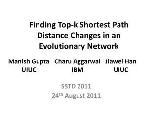
Finding Top-k Shortest Path Distance Changes in an Evolutionary Network

1. Finding Top-k Shortest Path Distance Changes in an Evolutionary Network Manish Gupta UIUC CharuAggarwal IBM Jiawei Han UIUC SSTD 2011 24th August 2011

2. Networks as evolutionary graphs • Social networks: new users join, new friendships are created. • Bibliographic networks: new authors publish more papers, more collaborations are done. • Transportation/road networks: new roads are constructed. • Ad hoc networks: Army vehicles change positions very frequently, new messages transmitted.

3. Analysis of evolutionary networks • Community formation, using clustering techniques • Metrics to study evolution – merge/split • Information diffusion across evolutionary networks • Link prediction tasks • Queries over evolving networks

4. Queries over Evolving networks • Updating shortest path distance between two nodes as the edge weights change. E.g., in computer networks, routers need to update their shortest path trees when a link goes down. • Given a time dependent network (edge weights are function of time), how to compute SPD(u, v, t). • Queries incorporating the max flow constraints.

5. Transportation Planning Problem • Given the current set of roads, we want to overlay a network of new roads. • Civil engineers propose two plans: A and B with different sets of new roads • Which plan is better? • Plan A brings cities X and Y very close. X produces a lot of product P while Y has a rich demand for product P. • Plan A actually brings lots of “economically important pairs” of cities close to each other. Select plan A over B.

6. Our problem • Given an evolutionary network with two snapshots G1 and G2. • Compute top few node pairs with maximum shortest path distance change across the two snapshots. • For example, across 2005 and 2011, distance between which pair of cities in Illinois decreased the most, thanks to the new roads built in this time period?

7. Naïve Approach • Compute shortest path distance between every pair of nodes for snapshot G1. • Compute shortest path distance between every pair of nodes for snapshot G2. • Compute distance change for every pair of nodes. • Sort the distance change vector • Return node pairs corresponding to the top few distance change values. • Highly inefficient solution!

8. Solution • We experiment on three datasets: DBLP co-authorship graph, IMDB co-starring graph and Ontario province road network. • Throw in more CPUs! • Shortest path algorithms are easily parallelizable. Run single source shortest path runs across thousands of machines. • On the Ontario road network dataset, it took around 400 CPU days! OR • Use our algorithm • Our methods are ~50-100X faster than baseline

9. Outline • Smartly choose a seed set of few source nodes to run single source shortest path algorithm from: Incidence Algorithm. • Improve the accuracy of Incidence Algorithm by intelligently expanding the seed set using Edge importance estimation algorithm. • Generalize the problem to a node ranking problem. • Suggest node ranking strategies. • Experimental results and analysis.

10. Incidence Algorithm • Maximum distance change will happen for node pairs consisting of nodes on which new edges or edges with changed weights are incident. • Let V’ be the set of nodes with new edges. • Algorithm: Run single source SPD algorithm from each node in V’ on both snapshots, compute difference (change), sortand return top k.

11. Is Incidence Algorithm accurate? • For top 1, yes. • But not for top k. (k!=1) • could be greaterthan . • Multiple edges can combine together and cause much more distance changes compared to that by just one edge. • Solution: To get better accuracy, expand the seed set.

12. How to expand the seed set (V’)? • Consider the neighbors of all the nodes currently in V’ as potential candidates. • Expand to a promising neighbor. • In particular, expand to a neighbor node a, if the edge that connects a to the current set V’ has relatively high importance, relative to other edges incident on node a. Terminate when top k node pairs don’t change. V’ V’ a a

13. Edge importance number • Importance number of an edge is the probability that the edge will lie on a randomly chosen shortest path tree in the graph. • How to compute edge importance number for edge e? • First find all shortest path trees and then find how many of such trees contain edge e. • Too expensive! As inefficient as the naïve solution itself! • Hence we compute estimate edge importance number using a randomized algorithm.

14. Edge Importance Estimation Algorithm • Randomly sample a few nodes from the graph. • Using each of these nodes S as source, obtain a shortest path tree T using an SPD algorithm (e.g. Dijkstra). • For each tree T, perform distance labeling. • Alternative Tight edge: An alternative edgewhich could replace an existent edge from T to give T’. • For each edge in T, obtain multiple T’by replacing a tight edge using an alternative tight edge. • Edge importance of an edge wrt T is proportional to the number of descendants. • Aggregate I(edge) across all different SPTs.

15. Generalizing the problem • Naïve solution: Use all nodes in both snapshots. • Incidence algorithm: Use only nodes in V’. • Generalized solution? • Node ranking problem. • Rank nodes such that running Dijkstra algorithm from just top few nodes provides high accuracy for “topK node pairs with max distance change problem”.

16. How to rank nodes? • Random: Randomly select nodes from the graph. • RandomNWNE: Randomly select nodes from seed set V’ (nodes with new edges). • Edge Weight Based Ranking (EWBR). • Edge Weight Change Based Ranking (EWCBR). 0.2 0.2 0.2 0.02 0.1 0.1 0.1 0.01 0.15 0.3 0.2 0.3 0.1

17. How to rank nodes? • Importance Number Based Ranking (INBR) • Importance Number Change Based Ranking (INCBR) • Ranking Using Edge Weight and Importance Numbers (RUEWIN) 0.2 0.2 0.2 0.02 0.1 0.1 0.1 0.5 0.75 0.3 0.2 0.3 0.1

18. How to rank nodes? • Clustering Based Ranking (CBR) • Clustering Based Ranking with Partitions (CBRP) • Inter-cluster edges are more important than intra-cluster edges.

19. Clustering Based Ranking • How to estimate the distance saved by an edge e joining nodes u and v in new snapshot? • Distance saved = weight of edge e minus the SPD(u,v) in old snapshot. • How to estimate SPD(u,v) in old snapshot? • SPD(u,v) in old snapshot SPD(u, Cu)+SPD(Cu, Cv)+SPD(Cv, v) where Cu and Cv are centers of clusters/partitions containing u and v respectively. • CBR: Randomly select K nodes in the graph, run Dijkstra from each of the K nodes. Rank edges and hence nodes. • CBRP: Similar to CBR except that first partition graph using some graph partitioning algorithm (e.g. METIS) and then randomly choose a node within each partition. • Over-estimates SPD(u.v) in old snapshot for intra-cluster edges but not a worry!

20. Experiments

34. Related work • Shortest path algorithms: Dijkstra [11], Shimbel [20], Johnson [15], Floyd, Warshall [14,21] • Router networks [8,22] • Outlier detection [5,13,18] • Time dependent shortest paths [25,26] • Dynamic shortest paths computation [3,4,6,19] • Between-ness measures [23,24]

36. References

37. References

38. References

39. Thanks!