Shortest Path Problems
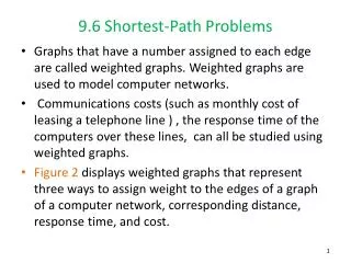
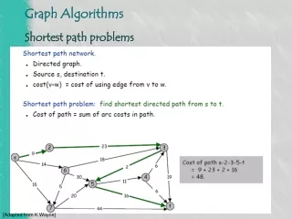
Shortest Path Problems . Bellman-Ford Algorithm for the Single-Source Shortest Path Problem with Arbitrary Arc Costs Updated 18 February 2008. Bellman-Ford Algorithm. begin d (i) := for each node i in N d ( s ) := 0 and pred( s ) := 0; for k = 1 to n


Shortest Path Problems
E N D
Presentation Transcript
Shortest Path Problems Bellman-Ford Algorithm for the Single-Source Shortest Path Problem with Arbitrary Arc Costs Updated 18 February 2008
Bellman-Ford Algorithm begin d(i) := for each node i in N d(s) := 0 and pred(s) := 0; for k = 1 to n for each (i, j) in A do if d(j) > d(i) + cijthen d(j) := d(i) + cijand pred(j) := i end;
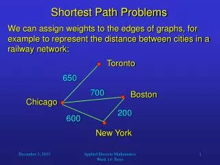
1 2 -2 1 1 3 4 3 Bellman-Ford Example 1 0 2
d1(1) = 0 d1(2) = -1 d1(3) = 4 d1(4) = 1 Bellman-Ford Example 1 0 -1 2 k =1 1 2 -2 1 1 3 4 3 4 1 dk(i) denotes d(i) after iteration k
d2(1)=0 d2(2)=-1 d2(3)=0 d2(4)=1 Bellman-Ford Example 1 -1 0 k = 2 2 1 2 -2 1 1 3 4 3 1 0 4
d3(1)=0 d3(2)=-1 d3(3)=0 d3(4)=1 Bellman-Ford Example 1 -1 0 k =3 2 1 2 -2 1 1 3 4 3 d3(i)= d2(i) 1 0
Shortest Path Tree -1 0 2 1 2 d(j) d(i) + cij and d(j) =d(i) + cij for all predecessor arcs -2 1 1 3 4 3 0 1
Complexity of Bellman-Ford • There are n iterations • Each iteration inspects each arc once • Inspecting an arc is O(1) • Complexity is O(mn)
Bellman-Ford Example 2 0 100 1 2 10 200 -150 -150 4 3
d1(1) = 0 d1(2) = 100 d1(3) = d1(4) = 200 Bellman-Ford Example 2 100 0 100 k = 1 1 2 10 -150 200 -150 4 3 200
d2(1) = 0 d2(2) = -100 d2(3) = 50 d2(4) = -90 Bellman-Ford Example 2 -100 100 100 0 100 k = 2 1 2 10 -150 200 -150 4 3 100 50 200 -90 100
d3(1) = 0 d3(2) = -100 d3(3) = -240 d3(4) = -90 Bellman-Ford Example 2 -100 0 100 k = 3 1 2 10 -150 200 -150 4 3 -90 -240 100 50
Bellman-Ford Example 2 -100 -390 0 100 k = 4 1 2 10 d4(1) = 0 -150 200 d4(2) = -390 d4(3) = -240 -150 4 3 d4(4) = -90 -90 -240 100 d3(2) = -100
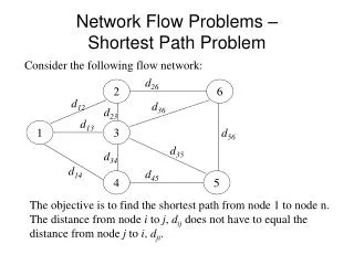
Detecting Negative-Cost Cycles • If there is a negative-cost cycle in G, then dn(i) < dn-1(i) for some node i.
Detecting Negative-Cost Cycles dn-1(1) dn-1(2) 1 2 dn(4) dn-1(1) + c14 dn(1) dn-1(2) + c21 dn(2) dn-1(3) + c32 4 3 dn(3) dn-1(4) + c43 dn-1(4) dn-1(3)
Detecting Negative-Cost Cycles If the length of the cycle < 0 then dn(i) < dn-1(i) for at least one node i in the cycle.