Shortest Path Problems
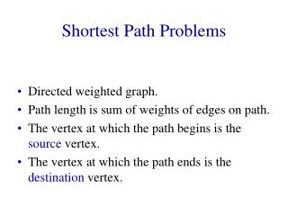
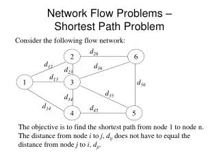
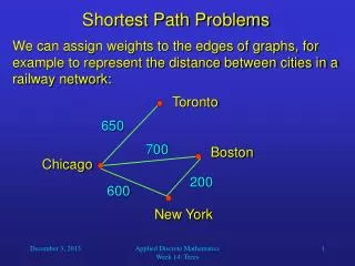
Toronto. 650. 700. Boston. Chicago. 200. 600. New York. Shortest Path Problems. We can assign weights to the edges of graphs, for example to represent the distance between cities in a railway network:. Shortest Path Problems.

Shortest Path Problems
E N D
Presentation Transcript
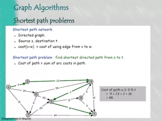
Toronto 650 700 Boston Chicago 200 600 New York Shortest Path Problems • We can assign weights to the edges of graphs, for example to represent the distance between cities in a railway network: Applied Discrete Mathematics Week 14: Trees
Shortest Path Problems • Such weighted graphs can also be used to model computer networks with response times or costs as weights. • One of the most interesting questions that we can investigate with such graphs is: • What is the shortest path between two vertices in the graph, that is, the path with the minimal sum of weights along the way? • This corresponds to the shortest train connection or the fastest connection in a computer network. Applied Discrete Mathematics Week 14: Trees
Dijkstra’s Algorithm • Dijkstra’s algorithm is an iterative procedure that finds the shortest path between to vertices a and z in a weighted graph. • It proceeds by finding the length of the shortest path from a to successive vertices and adding these vertices to a distinguished set of vertices S. • The algorithm terminates once it reaches the vertex z. Applied Discrete Mathematics Week 14: Trees
Dijkstra’s Algorithm • procedure Dijkstra(G: weighted connected simple graph with vertices a = v0, v1, …, vn = z and positive weights w(vi, vj), where w(vi, vj) = if {vi, vj} is not an edge in G) • for i := 1 to n • L(vi) := • L(a) := 0 • S := • {the labels are now initialized so that the label of a is zero and all other labels are , and the distinguished set of vertices S is empty} Applied Discrete Mathematics Week 14: Trees
Dijkstra’s Algorithm • while zS • begin • u := the vertex not in S with minimal L(u) • S := S{u} • for all vertices v not in S • if L(u) + w(u, v) < L(v) then L(v) := L(u) + w(u, v) • {this adds a vertex to S with minimal label and updates the labels of vertices not in S} • end{L(z) = length of shortest path from a to z} Applied Discrete Mathematics Week 14: Trees
b d a z c e Dijkstra’s Algorithm • Example: 5 6 4 8 1 2 0 3 2 10 Step 0 Applied Discrete Mathematics Week 14: Trees
b d 5 6 4 8 a 1 z 2 0 3 2 10 c e Dijkstra’s Algorithm 4 (a) • Example: 2 (a) Step 1 Applied Discrete Mathematics Week 14: Trees
b d 5 6 4 8 a 1 z 2 0 3 2 10 c e Dijkstra’s Algorithm 3 (a, c) 4 (a) 10 (a, c) • Example: 2 (a) 12 (a, c) Step 2 Applied Discrete Mathematics Week 14: Trees
b d 5 6 4 8 a 1 z 2 0 3 2 10 c e Dijkstra’s Algorithm 3 (a, c) 4 (a) 10 (a, c) 8 (a, c, b) • Example: 2 (a) 12 (a, c) Step 3 Applied Discrete Mathematics Week 14: Trees
b d 5 6 4 8 a 1 z 2 0 3 2 10 c e Dijkstra’s Algorithm 3 (a, c) 4 (a) 10 (a, c) 8 (a, c, b) • Example: 14 (a, c, b, d) 2 (a) 12 (a, c) 10 (a, c, b, d) Step 4 Applied Discrete Mathematics Week 14: Trees
b d 5 6 4 8 a 1 z 2 0 3 2 10 c e Dijkstra’s Algorithm 4 (a) 3 (a, c) 8 (a, c, b) 10 (a, c) • Example: 14 (a, c, b, d) 13 (a, c, b, d, e) 2 (a) 12 (a, c) 10 (a, c, b, d) Step 5 Applied Discrete Mathematics Week 14: Trees
b d 5 6 4 8 a 1 z 2 0 3 2 10 c e Dijkstra’s Algorithm 4 (a) 3 (a, c) 8 (a, c, b) 10 (a, c) • Example: 14 (a, c, b, d) 13 (a, c, b, d, e) 2 (a) 12 (a, c) 10 (a, c, b, d) Step 6 Applied Discrete Mathematics Week 14: Trees
The Traveling Salesman Problem • The traveling salesman problem is one of the classical problems in computer science. • A traveling salesman wants to visit a number of cities and then return to his starting point. Of course he wants to save time and energy, so he wants to determine the shortest path for his trip. • We can represent the cities and the distances between them by a weighted, complete, undirected graph. • The problem then is to find the circuit of minimum total weight that visits each vertex exactly once. Applied Discrete Mathematics Week 14: Trees
Toronto 650 550 700 Boston 700 Chicago 200 600 New York The Traveling Salesman Problem • Example: What path would the traveling salesman take to visit the following cities? Solution: The shortest path is Boston, New York, Chicago, Toronto, Boston (2,000 miles). Applied Discrete Mathematics Week 14: Trees
The Traveling Salesman Problem • Question: Given n vertices, how many different cycles Cn can we form by connecting these vertices with edges? • Solution: We first choose a starting point. Then we have (n – 1) choices for the second vertex in the cycle, (n – 2) for the third one, and so on, so there are (n – 1)! choices for the whole cycle. • However, this number includes identical cycles that were constructed in opposite directions. Therefore, the actual number of different cycles Cn is (n – 1)!/2. Applied Discrete Mathematics Week 14: Trees
The Traveling Salesman Problem • Unfortunately, no algorithm solving the traveling salesman problem with polynomial worst-case time complexity has been devised yet. • This means that for large numbers of vertices, solving the traveling salesman problem is impractical. • In these cases, we can use approximation algorithms that determine a path whose length may be slightly larger than the traveling salesman’s path, but can be computed with polynomial time complexity. • For example, artificial neural networks can do such an efficient approximation task. Applied Discrete Mathematics Week 14: Trees
Let us talk about… • Trees Applied Discrete Mathematics Week 14: Trees
Trees • Definition: A tree is a connected undirected graph with no simple circuits. • Since a tree cannot have a simple circuit, a tree cannot contain multiple edges or loops. • Therefore, any tree must be a simple graph. • Theorem: An undirected graph is a tree if and only if there is a unique simple path between any of its vertices. Applied Discrete Mathematics Week 14: Trees
Trees • Example: Are the following graphs trees? Yes. No. No. Yes. Applied Discrete Mathematics Week 14: Trees
Trees • Definition: An undirected graph that does not contain simple circuits and is not necessarily connected is called a forest. • In general, we use trees to represent hierarchical structures. • We often designate a particular vertex of a tree as the root. Since there is a unique path from the root to each vertex of the graph, we direct each edge away from the root. • Thus, a tree together with its root produces a directed graph called a rooted tree. Applied Discrete Mathematics Week 14: Trees
Tree Terminology • If v is a vertex in a rooted tree other than the root, the parent of v is the unique vertex u such that there is a directed edge from u to v. • When u is the parent of v, v is called the child of u. • Vertices with the same parent are called siblings. • The ancestors of a vertex other than the root are the vertices in the path from the root to this vertex, excluding the vertex itself and including the root. Applied Discrete Mathematics Week 14: Trees
Tree Terminology • The descendants of a vertex v are those vertices that have v as an ancestor. • A vertex of a tree is called a leaf if it has no children. • Vertices that have children are called internal vertices. • If a is a vertex in a tree, then the subtree with a as its root is the subgraph of the tree consisting of a and its descendants and all edges incident to these descendants. Applied Discrete Mathematics Week 14: Trees
Tree Terminology • The level of a vertex v in a rooted tree is the length of the unique path from the root to this vertex. • The level of the root is defined to be zero. • The height of a rooted tree is the maximum of the levels of vertices. Applied Discrete Mathematics Week 14: Trees
Trees James • Example I: Family tree Christine Bob Frank Joyce Petra Applied Discrete Mathematics Week 14: Trees
Trees / • Example II: File system usr bin temp bin spool ls Applied Discrete Mathematics Week 14: Trees
Trees • Example III: Arithmetic expressions + - y z x y This tree represents the expression (y + z)(x - y). Applied Discrete Mathematics Week 14: Trees
Trees • Definition: A rooted tree is called an m-ary tree if every internal vertex has no more than m children. • The tree is called a full m-ary tree if every internal vertex has exactly m children. • An m-ary tree with m = 2 is called a binary tree. • Theorem: A tree with n vertices has (n – 1) edges. • Theorem: A full m-ary tree with i internal vertices contains n = mi + 1 vertices. Applied Discrete Mathematics Week 14: Trees