Universality

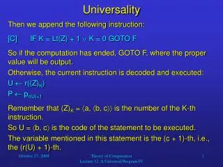
1. Universality Then we append the following instruction: [C] IF K = Lt(Z) + 1  K = 0 GOTO F So if the computation has ended, GOTO F, where the proper value will be output. Otherwise, the current instruction is decoded and executed: U  r((Z)K) P  pr(U)+1 Remember that (Z)K = a, b, c is the number of the K-th instruction. So U = b, c is the code of the statement to be executed. The variable mentioned in this statement is the (c + 1)-th, i.e., the (r(U) + 1)-th. Theory of Computation Lecture 12: A Universal Program IV

2. Universality Then l(U) contains the type of the instruction to be executed. IF l(U) = 0 GOTO N IF l(U) = 1 GOTO A IF (P | S) GOTO N IF l(U) = 2 GOTO M If either the instruction is V  V, or the instruction is V  V-1 and V = 0 (as indicated by the absence of P in S), or the instruction is IF V0 GOTO L and V = 0, then nothing is done to S (“nothing” - GOTO N). If the instruction is V  V+1, then the exponent of P in S needs to be incremented (“add” – GOTO A). If the instruction is V  V-1 with V > 0, then the exponent of P in S needs to be decremented (“minus” – GOTO M). Theory of Computation Lecture 12: A Universal Program IV

3. If none of the four previous predicates were true, a GOTO command has to be executed: K  miniLt(Z) [l((Z)i) + 2 = l(U)] GOTO C So if the label l(U) – 2 exists in the program, the number K of the next instruction to be executed will be set to the first instruction with that label. Otherwise, K will be set to 0. As you remember, if K = 0 or K = Lt(Z) + 1, then the computation stops. In any case, our interpreter program executes a GOTO C to execute the next instruction. Universality Theory of Computation Lecture 12: A Universal Program IV

4. Universality The program continues as follows: [M] S  S/P GOTO N [A] S  S  P [N] K  K+1 GOTO C The value of the variable in the current instruction is decremented or incremented by 1 by dividing or multiplying S by P, respectively. Then K is incremented and the next instruction executed. Theory of Computation Lecture 12: A Universal Program IV

5. Universality The program concludes with the following line: [F] Y  (S)1 This way, after termination of the interpreted program, its output value becomes the output value of the interpreter. On the next slide, we will list the entire interpreter program. Theory of Computation Lecture 12: A Universal Program IV

6. Universality Z  Xn+1 + 1 S  ni=1 (p2i)Xi K  1 [C] IF K = Lt(Z) + 1  K = 0 GOTO F U  r((Z)K) P  pr(U)+1 IF l(U) = 0 GOTO N IF l(U) = 1 GOTO A IF (P | S) GOTO N IF l(U) = 2 GOTO M K  miniLt(Z) [l((Z)i) + 2 = l(U)] GOTO C [M] S  S/P GOTO N [A] S  S  P [N] K  K+1 GOTO C [F] Y  (S)1 Theory of Computation Lecture 12: A Universal Program IV

7. Universality For each n > 0, the sequence (n)(x1, …, xn, 0), (n)(x1, …, xn, 1), … enumerates all partially computable functions of n variables. We can also write: y(n)(x1, …, xn) = (n)(x1, …, xn, y). We can omit the superscript (n) when n = 1: y(x) = (x, y) = (1)(x, y). Theory of Computation Lecture 12: A Universal Program IV

8. Universality Consider the following predicates: STP(n)(x1, …, xn, y, t)  Program number y halts after t or fewer steps on inputs x1, …, xn  There is a computation of program y of length  t + 1, beginning with inputs x1, …, xn These predicates are computable, which we can easily prove: We can simply add a counter to our universal programs to determine when we have simulated t steps. Theory of Computation Lecture 12: A Universal Program IV

9. Universality Consider the following predicates: STP(n)(x1, …, xn, y, t)  Program number y halts after t or fewer steps on inputs x1, …, xn  There is a computation of program y of length  t + 1, beginning with inputs x1, …, xn These predicates are computable, which we can easily prove: We can simply add a counter to our universal programs to determine when we have simulated t steps. Theory of Computation Lecture 12: A Universal Program IV

10. Universality We can prove an even stronger theorem: Theorem 3.2 (Step-Counter Theorem): For each n > 0, the predicate STP(n)(x1, …, xn, y, t) is primitive recursive. Proof: We will provide numerical descriptions of the notions of snapshot and successor snapshot. This will show that the necessary functions are primitive recursive. See pages 74 and 75 in the textbook for the proof. Theory of Computation Lecture 12: A Universal Program IV

11. Universality Now that we know the Step-Counter Theorem, we are ready for yet another theorem. Proving this theorem will be similar to the last one. Theorem 3.3 (Normal Form Theorem): Let f(x1, …, xn) be a partially computable function. Then there is a primitive recursive predicate R(x1, …, xn, y) such that f(x1, …, xn) = l(minz R(x1, …, xn, z)) Theory of Computation Lecture 12: A Universal Program IV

12. Universality Proof: Let y0 be the number of a program that computes f(x1, …, xn). Then consider the equation f(x1, …, xn) = l(minz R(x1, …, xn, z)) , where R(x1, …, xn, z) is the predicate STP(n) (x1, …, xn, y0, r(z))& (r(SNAP(n) (x1, …, xn, y0, r(z))))1 = l(z) If the right side of the first equation is defined, then there exists a number z such that STP(n) (x1, …, xn, y0, r(z)) and (r(SNAP(n) (x1, …, xn, y0, r(z))))1 = l(z) Theory of Computation Lecture 12: A Universal Program IV

13. Universality • For any such z, • the computation by the program with number y0 has reached a terminal snapshot in r(z) or fewer steps, • l(z) is the value of the output variable Y, that is, l(z) = f(x1, …, xn). • If the right side of the equation is undefined, it must be true that STP(n) (x1, …, xn, y0, t) is false for all values of t, that is, f(x1, …, xn) is undefined. Theory of Computation Lecture 12: A Universal Program IV

14. Universality Theorem 3.4: A function is partially computable if and only if it can be obtained from the initial functions by a finite number of applications of composition, recursion, and minimalization. Proof: It follows from Theorems 1.1, 2.1, 2.2, 3.1, and 7.2 in Chapter 3 that every function that can be so obtained is partially computable. Theory of Computation Lecture 12: A Universal Program IV

15. Universality Now let us consider the “opposite direction” of the Normal Form Theorem (Theorem 3.3): We can use the normal form theorem to write any given partially computable function in the form l(miny R(x1, …, xn, y)) , where R is a primitive recursive predicate and therefore is obtained from the initial functions by a finite number of applications of composition and recursion. Finally, our given function is obtained from R by one use of minimalization and then by composition with the primitive recursive function l. Theory of Computation Lecture 12: A Universal Program IV

16. Universality When miny R(x1, …, xn, y)) is a total function (that is, when for each x1, …, xn there is at least one y for which R(x1, …, xn, y) is true), we say that we are applying the operation of proper minimalization to R. Now, if l(miny R(x1, …, xn, y)) is total, then miny R(x1, …, xn, y) must be total. This gives us the following theorem: Theorem 3.5: A function is computable if and only if it can be obtained from the initial functions by a finite number of applications of composition, recursion, and proper minimalization. Theory of Computation Lecture 12: A Universal Program IV

17. Recursively Enumerable Sets From previous classes, such as CS 320, you may remember the correspondence between predicates and sets. We now want to use the set notation in our discussion of solvable and unsolvable problems. For example, the predicate HALT(x, y) is the characteristic function of the set {(x, y)  N2 | HALT(x, y)}. We say that a set B  Nm belongs to some class of functions if and only if the characteristic function P(x1, …, xn) of B belongs to the class in question. Theory of Computation Lecture 12: A Universal Program IV

18. Recursively Enumerable Sets Thus, saying that a set B is computable or recursive is the same as saying that P(x1, …, xn) is a computable function. Likewise, B is a primitive recursive set if P(x1, …, xn) is a primitive recursive predicate. It follows that: Theorem 4.1: Let the sets B, C belong to some PRC class C . Then so do the sets BC, BC, B. Proof: This is an immediate consequence of Theorem 5.1, Chapter 3. Theory of Computation Lecture 12: A Universal Program IV