Download
1 / 18
180 likes | 308 Vues
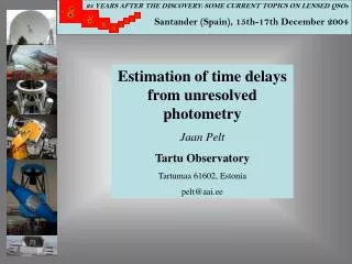
25 YEARS AFTER THE DISCOVERY: SOME CURRENT TOPICS ON LENSED QSOs Santander (Spain), 15th-17th December 2004. Estimation of time delays from unresolved photometry Jaan Pelt Tartu Observatory Tartumaa 61602, Estonia pelt@aai.ee. Abstract.

E N D
25 YEARS AFTER THE DISCOVERY: SOME CURRENT TOPICS ON LENSED QSOs Santander (Spain), 15th-17th December 2004 Estimation of time delays from unresolved photometry Jaan Pelt Tartu Observatory Tartumaa 61602, Estonia pelt@aai.ee
Abstract • Long time monitoring of the gravitational lens systems often proceeds using telescopes and recording equipment with modest resolution. • From high resolution images we know that the obtained quasar images are often blends and the corresponding time series are not pure shifted replicas of the source variability (let us forget about microlensing for a moment). • It occurs, that using proper statistical methods, we can still unscramble blended light curves and compute correct time delays. • We will show how to use dispersion spectra to compute two independent delays from A,B1 + B2 photometry and in the case of high quality photometry even more delays from truly complex systems. • In this way we can significantly increase the number of gravitational lens systems with multiple images for which a full set of time delays can be estimated.
Relevant persons: Sjur, Rudy, Jan and Jan-Erik (author’s photo)
Unresolved photometry, a problem for many systems An I-filter direct image of PG 1115+080 showing QSO components A1, A2, B, and C circa 28 authors, ApJ 475:L85-L88
Weighted sums of the two signals can be computed using similar expressions for pairs Dispersion spectra
Simple (oversimplified) algorithm to analyze unresolved photometry. • Assume that A signal is a pure source signal. ( A(t) = g(t) ). • 2. Assume that B signal is a sum of two pure source signals, both of them shifted in time by certain, but different, amounts. • B = B1+B2 = g(t-Delay)+g(t-Delay+Shift). • 3. To seek proper values for the Delay and Shift we can build for certain trial value of Shift a matching curve M(t) from A(t).M(t) = A(t)+A(t+Shift). The value for the Delay can now be estimated (for this particular Shift) by using standard methods with M(t) and B(t) as input data. For every trial Shift we will have a separate dispersion spectrum and putting all together we will have a two-dimensional dispersion surface.
Two model curves computed from a single random walk sequence. Upper curve is a sum of shifted and original sequence.
Model data with Delay = 12 and Shift = -5 (or Delay = 17 and Shift = 5), Scatter = 0%
Sign for the delay can be easily seen. The significant minima occur only on the right side of the diagram. Delay = 12 and Shift = -5, Scatter = 0%, Dispersion is on logarithmic scale.
Which of the curves is a blend can be also detected by exchanging A and B curves. Now there are four strong minima on the left side of the dispersion surface. Delay = -17 and Shift = -5, Scatter = 0%.
Scatter = 2% Scatter = 5% Scatter = 10% Scatter = 20% The two dimensional spectra depend on noise level of the input curves. However, as seen from the plots, there is a quite large “working” region for the method.
Real data. Celebrated double quasar. PSF analysis by Ovaldsen from Schild data. B curve is shifted left by 417 days and down by 0.1 mag.
Double quasar data. Delay = 424 Shift = 32. Dispersion = 0.548. B = B1+B2
Double quasar data. Delay = -415 Shift = 24. Dispersion = 0.375. A = A1+A2
Simplifications. • We ignored different levels of noise for the true signals and for the combined signals. • We assumed that B1 and B2 (or A1 and A2) are of equal strength. • 3. Only the case A, B1+B2 (or B, A1+A2) was considered, but what about A1+A2, B1+B2 case (if physically feasible)?
Conclusions • The methods based on dispersion spectra can be applied to unresolved photometry. • The amount of computations is raised significantly, especially if we analyze blends with unequal strength. In these cases the spectra will have already three dimensions. • To validate proposed methodology we need photometric data sets with good time coverage, low noise level and, if possible, well established geometry (from high resolution imaging). • The real data sets (in our case the celebrated double quasar) can show complex behavior which can not be yet easily interpreted. • Proposals are welcome: pelt@aai.ee
If all this seemed to be too messy, then I can tell you, it was as messy as Mother Nature in Estonia!