Chap8: Trends in DBMS
190 likes | 385 Vues
Chap8: Trends in DBMS. 8.1 Database support for Field Entities 8.2 Content-based retrieval 8.3 Introduction to spatial data warehouses 8.4 Summary. Learning Objectives. Learning Objectives (LO) LO1: Learn about field data LO2 : Learn about storage and retrieval of field data

Chap8: Trends in DBMS
E N D
Presentation Transcript
Chap8: Trends in DBMS 8.1 Database support for Field Entities 8.2 Content-based retrieval 8.3 Introduction to spatial data warehouses 8.4 Summary
Learning Objectives • Learning Objectives (LO) • LO1: Learn about field data • LO2 : Learn about storage and retrieval of field data • LO3: Learn about spatial data warehouses • What are data warehouses? Why are they interesting? • What are aggregate functions? Which ones are easy to compute? • Mapping Sections to learning objectives • LO1 - 8.1 • LO2 - 8.1.2, 8.2 • LO3 - 8.3
8.3 Why are Data Warehouses Interesting? • Data Warehouse facilitate group decision making • Consider a dataset • 1 measure (i.e. Sales) • 3 dimensions (e.g. Company, Year, Region) • Analysis questions • Q1. Rank Regions by total sales. • Q2. Rank years by total sales. • Q3. Where are sales consistently growing? • Cross tabulates summaries reports used to analyze the trends • Example:
8.3 Generating cross-tabulation summaries • TraditionalApproach • Use custom software pulling data out of a DBMS • Limitations: redundant of work, inefficient use of resources • Data Warehouse approach • Cross-tab. Can be generated using a set of simple report • Each report is generated from a SQL “Select ... group by” statement • Example: Fig. 8.19 (pp. 244) and Table 8.3 (pp. 245) • Cross-tab example in last slide is a union of • SALES-L0-A, SALES-L1-A, SALES-L1-B and SALES-L2 • Table 8.3 shows SQL queries to compute each part • Advantage • Rest of SQL is available for pre/post processing of data • Performance gains by eliminating unnecessary copying of data
Example Data Warehouse (Fig. 8.19) Fig 8.19
8.3.4 Cross-tabulation vs.report hierarchy • Spreadsheet view of a report • Views a report a N-dim. Spreadsheet • N = number of dimension attributes • Each cell contains value of “measure” • Cross-tabulation view of a Report hierarchy • Example: report hierarchy for • SALES-L0-A, SALES-L2-A, SALES-L1-B, SALES-L2, Fig. 8.19 (pp. 244)
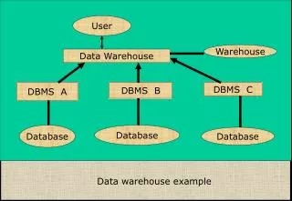
8.3 What is a Data Warehouse? • Data Warehouse is a special purpose database • Primarily used for specialized data analysis purposes • Facilitates generation and navigation of a hierarchy of reports • Special purpose data-sets and queries • Data consists of • a few measure attributes • a set of dimension attributes • The measure attribute depends on dimension attributes • Queries generate reports • Report measure for selected values of dimensions • Aggregate measure for given subset of dimensions • What is a spatial data warehouse? • Data warehouses with spatial measures or dimensions • Example: census data - census tract is a spatial dimension • Example: logistics data - route is a spatial dimension
8.3.4 Data Warehouse Operations • Operations on a data warehouse • Roll-up, Drill-down • Slice, Dice • Pivot • Roll-up • Inputs: A report R, A subset S of dimensions in R • Output: A sequence of reports summarizing R • Example 1: R = SALES-Base, S = (Year, Region) in Fig. 8.19 (pp. 244) • Output consists of reports SALES-L0-A, SALES-L1-B, SALES-L2 • Example 2: R = SALES-Base, S = (Region, Year) • Output consists of reports SALES-L0-A, SALES-L1-A, SALES-L2 • Drill-down • Inputs: A report R, A dimension D not in R • Output: A reports detailing R on D • Example: R = SALES-L1-B, D = Region in Fig. 8.19 (pp. 244) • Output : report SALES-L0-A
8.3.4 Data Warehouse Operations • Slice, Dice • Reduce dimensions in a table- (Fig. 8.7, pp 232). • Inputs: A report R, A value V for a dimension D in R • Output: A subset of R where D =V • Example: R = SALES-L0-A, D = Year, V = 1994 in Fig. 8.19 (pp. 244) • Output: Table 8.5 (pp. 246) • includes tuple (ALL, 1994, America, 35) Fig 8.7
8.3.4 Data Warehouse Operations • Pivot • For a spreadsheet view of reports • Transposes a spreadsheet • Example • Inputs: A spreadsheet view of a report R • Output: A transposed spreadsheet • Ex.: R= SALES-L0-A, Fig. 8.19 (pp. 244)
Logical Data Model of a DWH • Purpose of a logical data model • Specify a framework to specify computational structure • Allow extension of SQL to model new needs • Cube operation • Input : A fact table • Output: A set of summary reports covering all subsets of dimension columns • Equivalent to union of all tables and reports in Fig. 8.19 (pp. 244) • Ex. Fig. 8.18, pp. 243 • SELECT Company, Year, Region, Sum(Sales) AS Sales • FROM SALES • GROUP BY CUBE Company, Year, Region
Physical Data Model of a DWH • Purpose: Computationally efficient implementation • Ideas: • Pre-computation - • pre-compute some of reports and use those to compute other reports • New indexing methods, e.g. bit-map index • Query Processing Strategies • Strategies for aggregate functions • New strategies for multi-table joins • Let us look at strategies for aggregate functions
DWH Physical Model: Aggregate function strategies • Aggregate Functions • Compute summary statistics for a given set of values • Examples: sum, average, centroid (Table 8.1, pp. 238) • Strategies for efficient computation • Characterize easy to compute aggregate functions • 3 categories • Distributive • Algebraic • Holistic • First 2 categories can be computed easily in one scan of the dataset
Definitions of Aggregate Function Categories • Notation: • F, G, G1, G2, … Gn are aggregate functions where n is small • S is a set of values, e.g. S = (1, 2, 3, 4) • P = (S1, S2, …, Sp) is a partition of S, e.g. P = (S1, S2), S1 = (1, 2), S2 = (3, 4) • Distributive( F ) if there exists a G such that • F( S ) = G ( F(S1), F(S2), …, F(Sn) ) • Example: sum is distributive • Illustration: sum(1, 2, 3, 4) = sum ( sum(1, 2), sum(3, 4) • Algebraic( F ) if there exists G1, …, Gn, (where n is small) and • F( S ) = G ( G1(S1), …, Gn(S1), G2(S1), …, Gn(S2), …, G1(Sp), …, Gn(Sp) ) • Example: average is distributive • Illustration: average(1, 2, 3, 4) • = { count(1, 2) * average(1, 2) + count(3, 4) * average } / { count(1,2) + count(3,4) }
Example: Distributive Aggregate Function • Examples in cross-tabulation scenario (Fig. 8.14, pp.238): • Example 1. Min is distributive • Example 2. Count is distributive Fig 8.14
Examples: Algebraic Aggregate Functions • Examples in cross-tabulation scenario (Fig. 8.15, pp.239): • Average and Variance are algebraic Fig 8.15
Discussion - Spatial Data Warehouse • Example • Consider the example in Fig. 8.16, pp. 241 • A map interpretation may be attached to each report • Each row has a spatial footprint, which can be aggregated by geometric-union • The collection of maps may be called a mapcube • Issues: • What is needed in OGIS standard to support map-cube operation? • Hierarchical collection of maps in mapcube • What is an appropriate cartography to convey the relationship among maps?
Spatial Data Warehouses and Mapcube Fig 8.16
Summary • Field data • useful in many applications due to rich content • Represented as raster or image • Operations can be categorized into local, focal, zonal, and global • Field data storage and retrieval • Tiling is a preferred way to divide raster data into disk blocks • Meta-data based query is often used for retrieval • Content based retrieval may be used for similarity searches • Data warehouses support analysis e.g. cross-tabulation reports • SQL CUBE operator support generation of DWH reports • Distributive and Algebraic aggregate functions can be computed easily