Indices in a DBMS
1.27k likes | 1.62k Vues
Indices in a DBMS. Organization of Records in Files. Heap – a record can be placed anywhere in the file where there is space Sequential – store records in sequential order, based on the value of the search key of each record

Indices in a DBMS
E N D
Presentation Transcript
Organization of Records in Files Heap– a record can be placed anywhere in the file where there is space Sequential – store records in sequential order, based on the value of the search key of each record Hashing – a hash function computed on some attribute of each record; the result specifies in which block of the file the record should be placed Records of each relation may be stored in a separate file. In a clustering file organization records of several different relations can be stored in the same file Motivation: store related records on the same block to minimize I/O
Index Classification Primary vs. Secondary primary– the index on the primary key unique– an index on a candidate key secondary– not primary Clustered vs Unclustered clustered – key order corresponds with record order E.g. B-tree separate from record file Index-organized table B-tree leaves store records (no file) unclustered – index contains record-IDs in random order
Root B+Tree n=4 100 120 150 180 30 3 5 11 120 130 180 200 100 101 110 150 156 179 30 35
Sample non-leaf to keys to keys to keys to keys < 57 57 k<81 81k<95 95 57 81 95
Sample leaf node: From non-leaf node to next leaf in sequence 57 81 95 To record with key 57 To record with key 81 To record with key 85
Non-root nodes have to be at least half-full Use at least Non-leaf: n/2 children Leaf: (n-1)/2 pointers to data
Full node min. node Non-leaf Leaf n=4 120 150 180 30 3 5 11 30 35
Insert into B+tree (a) simple case space available in leaf (b) leaf overflow (c) non-leaf overflow (d) new root
(simple case) Insert key = 32 32 n=4 100 30 3 5 11 30 31
(leaf overflow) Insert key = 7 7 3 5 7 n=4 100 30 3 5 11 30 31
(internal overflow) Insert key = 160 160 180 160 179 n=4 100 120 150 180 180 200 150 156 179
(new root) insert 45 30 new root 40 40 45 n=4 10 20 30 1 2 3 10 12 20 25 30 32 40
insert: 1, 2, 10, 20, 3, 12, 30, 32, 25, 40, 45 n=4
(a) Simple case - no example (b) Coalesce with neighbor (sibling) (c) Re-distribute keys (d) Cases (b) or (c) at non-leaf Deletion from B+tree
(b) Coalesce with sibling Delete 50 40 n=5 10 40 100 10 20 30 40 50
(c) Redistribute keys Delete 50 35 35 n=4 10 40 100 20 30 35 40 50
new root 25 (d) Non-leaf coalesce • Delete 37 n=4 25 20 30 25 26 30 37 10 14 20 22 30
new root 25 (d) Non-leaf coalesce • Delete 37 n=4 25 20 30 25 26 30 37 10 14 20 22 30
B+tree deletions in practice Often, coalescing is not implemented Too hard and not worth it!
Interesting problem: For B+tree, how large should n be? … n is number of keys / node
Assumptions You have the right to set the disk page size for the disk where a B-tree will reside. Compute the optimum page size n assuming that The items are 4 bytes long and the pointers are also 4 bytes long. Time to read a node from disk is 10+.0002n Time to process a block in memory is unimportant B+tree is full (I.e., every page has the maximum number of items and pointers
FIND nopt by f’(n) = 0 What happens to nopt as • Disk bandwidth increases? • Access time stays behind? • CPU get faster?
f(n) = time to find a record = logn(T) * (10 + 0.0002n) 1994 (book) 2004 (now) N=500 n=4000
f(n) = time to find a record = logn(T) * (10 + 0.0002n) 1994 Table 1M records 10ms access time 4MB/s bandwidth n~500-1000 4KB / 8KB pages Be conservative to limit RAM consumption
f(n) = time to find a record = logn(T) * (10 + 0.0002n) 2004 Table 10M records 6ms access time 40MB/s bandwidth n~1000-4000 8KB / 32KB pages relative benefit decreases so don’t overdo it
FIND nopt by f’(n) = 0 Answer should be nopt = “few thousand” What happens to nopt as block sizes are increasing.. • Disk bandwidth increases? • Access time stays behind? • CPU get faster?
Primary or Auxiliary Structure • Primary index • Leaf blocks in sequence clustered index • Main storage structure for a database table • E.g. B+-tree organized file / hash structured files • Typically an index on an unique key • But not necessarily • Normally, you can have only one clustered index! • Secondary index • Also called unclustered index • A separate file from where the table is stored • Refers with (block/offset) pointers to records in the table file • You can define many as you want (to maintain)
Clustered vs. Unclustered Index Primary B-Tree index • Primary index • Leaf blocks in sequence clustered index • Main storage structure for a database table • E.g. B+-tree organized file / hash structured files • Typically an index on an unique key • But not necessarily • Normally, you can have only one clustered index! • Secondary index • Also called unclustered index • A separate file from where the table is stored • Refers with (block/offset) pointers to records in the table file • You can define many as you want (to maintain) low high 1 access only (rest is ‘just’ bandwidth)
Clustered vs. Unclustered Index Primary B-Tree index • Primary index • Leaf blocks in sequence clustered index • Main storage structure for a database table • E.g. B+-tree organized file / hash structured files • Typically an index on an unique key • But not necessarily • Normally, you can have only one clustered index! • Secondary index • Also called unclustered index • A separate file from where the table is stored • Refers with (block/offset) pointers to records in the table file • You can define many as you want (to maintain) low high 1 access only (rest is ‘just’ bandwidth) Pay N times access cost Secondary B-tree index
Are Unclustered Indices a Good Idea? • Secondary indices depend on random I/O • can do asynchronous I/O (multiple I/Os at-a-time) • degenerates into full table scans
Are Unclustered Indices a Good Idea? • Secondary indices depend on random I/O • can do asynchronous I/O (multiple I/Os at-a-time) • degenerates into full table scans • Is not using an index at all better? • I.e. read the entire table sequentially without any index • Use redundant clustered orderings • Materialized views • C-STORE (Stonebraker et al, VLDB 2005), MonetDB/X100 • Database Cracking (Kersten, CIDR 2005+2007)
Raster data consist of bit maps or pixel maps, in two or more dimensions. Example 2-D raster image: satellite image of cloud cover, where each pixel stores the cloud visibility in a particular area. Additional dimensions might include the temperature at different altitudes at different regions, or measurements taken at different points in time. Design databases generally do not store raster data. Geographic Data
Vector data are constructed from basic geometric objects: points, line segments, triangles, and other polygons in two dimensions, and cylinders, speheres, cuboids, and other polyhedrons in three dimensions. Vector format often used to represent map data. Roads can be considered as two-dimensional and represented by lines and curves. Some features, such as rivers, may be represented either as complex curves or as complex polygons, depending on whether their width is relevant. Features such as regions and lakes can be depicted as polygons. Geographic Data (Cont.)
Examples of geographic data map data for vehicle navigation distribution network information for power, telephones, water supply, and sewage Vehicle navigation systems store information about roads and services for the use of drivers: Spatial data: e.g, road/restaurant/gas-station coordinates Non-spatial data: e.g., one-way streets, speed limits, traffic congestion Global Positioning System (GPS) unit - utilizes information broadcast from GPS satellites to find the current location of user with an accuracy of tens of meters. increasingly used in vehicle navigation systems as well as utility maintenance applications. Applications of Geographic Data
Spatial Access • Develop a data structure to speedup spatial data access • Nearness queries request objects that lie near a specified location. • Nearest neighbor queries, given a point or an object, find the nearest object that satisfies given conditions. • Region queries deal with spatial regions. e.g., ask for objects that lie partially or fully inside a specified region. • Queries that compute intersections or unions of regions. • Spatial join of two spatial relations with the location playing the role of join attribute.
k-d tree - early structure used for indexing in multiple dimensions. Each level of a k-d tree partitions the space into two. choose one dimension for partitioning at the root level of the tree. choose another dimensions for partitioning in nodes at the next level and so on, cycling through the dimensions. In each node, approximately half of the points stored in the sub-tree fall on one side and half on the other. Partitioning stops when a node has less than a given maximum number of points. The k-d-B tree extends the k-d tree to allow multiple child nodes for each internal node; well-suited for secondary storage. Indexing of Spatial Data
Each line in the figure (other than the outside box) corresponds to a node in the k-d tree the maximum number of points in a leaf node has been set to 1. The numbering of the lines in the figure indicates the level of the tree at which the corresponding node appears. Division of Space by a k-d Tree
Quadtrees Each node of a quadtree is associated with a rectangular region of space; the top node is associated with the entire target space. Each non-leaf nodes divides its region into four equal sized quadrants correspondingly each such node has four child nodes corresponding to the four quadrants and so on Leaf nodes have between zero and some fixed maximum number of points (set to 1 in example). Division of Space by Quadtrees
Region quadtrees store array (raster) information. A node is a leaf node if all the array values in the region that itcovers are the same. Otherwise, it is subdivided further into four children of equal area, and is therefore an internal node. Each node corresponds to a sub-array of values. The sub-arrays corresponding to leaves either contain just a single array element, or have multiple array elements, all of which have the same value. Extensions of k-d trees and quadtrees have been proposed to index line segments and polygons Require splitting segments/polygons into pieces at partitioning boundaries Same segment/polygon may be represented at several leaf nodes Quadtrees (Cont.)
R-trees are a N-dimensional extension of B+-trees, useful for indexing sets of rectangles and other polygons. Supported in “many” modern database systems, along with variants like R+ -trees and R*-trees. Basic idea: generalize the notion of a one-dimensional interval associated with each B+ -tree node to an N-dimensional interval, that is, an N-dimensional rectangle. Will consider only the two-dimensional case (N = 2) generalization for N > 2 is straightforward, although R-trees work well only for relatively small N R-Trees
A rectangular bounding box is associated with each tree node. Bounding box of a leaf node is a minimum sized rectangle that contains all the rectangles/polygons associated with the leaf node. The bounding box associated with a non-leaf node contains the bounding box associated with all its children. Bounding box of a node serves as its key in its parent node (if any) Bounding boxes of children of a node are allowed to overlap A polygon is stored only in one node, and the bounding box of the node must contain the polygon The storage efficiency or R-trees is better than that of k-d trees or quadtrees since a polygon is stored only once R Trees (Cont.)
A set of rectangles (solid line) and the bounding boxes (dashed line) of the nodes of an R-tree for the rectangles. The R-tree is shown on the right. Example R-Tree
To find data items (rectangles/polygons) intersecting (overlaps) a given query point/region, do the following, starting from the root node: If the node is a leaf node, output the data items whose keys intersect the given query point/region. Else, for each child of the current node whose bounding box overlaps the query point/region, recursively search the child Can be very inefficient in worst case since multiple paths may need to be searched but works acceptably in practice. Simple extensions of search procedure to handle predicates contained-in and contains Search in R-Trees
Insertion in R-Trees • To insert a data item: • Find a leaf to store it, and add it to the leaf • To find leaf, follow a child (if any) whose bounding box contains bounding box of data item, else child whose overlap with data item bounding box is maximum • Handle overflows by splits (as in B+ -trees) • Split procedure is different though (see below) • Adjust bounding boxes starting from the leaf upwards • Split procedure: • Goal: divide entries of an overfull node into two sets such that the bounding boxes have minimum total area • This is a heuristic. Alternatives like minimum overlap are possible • Finding the “best” split is expensive, use heuristics instead • See next slide
Splitting an R-Tree Node • Quadratic split divides the entries in a node into two new nodes as follows • Find pair of entries with “maximum separation” • that is, the pair such that the bounding box of the two would has the maximum wasted space (area of bounding box – sum of areas of two entries) • Place these entries in two new nodes • Repeatedly find the entry with “maximum preference” for one of the two new nodes, and assign the entry to that node • Preference of an entry to a node is the increase in area of bounding box if the entry is added to the other node • Stop when half the entries have been added to one node • Then assign remaining entries to the other node • Cheaper linear split heuristic works in time linear in number of entries, • Cheaper but generates slightly worse splits.
Deleting in R-Trees • Deletion of an entry in an R-tree done much like a B+-tree deletion. • In case of underful node, borrow entries from a sibling if possible, else merging sibling nodes • Alternative approach removes all entries from the underfull node, deletes the node, then reinserts all entries