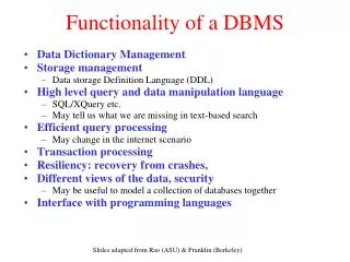
Functionality of a DBMS
Functionality of a DBMS. Data Dictionary Management Storage management Data storage Definition Language (DDL) High level query and data manipulation language SQL/XQuery etc. May tell us what we are missing in text-based search Efficient query processing May change in the internet scenario

Functionality of a DBMS
E N D
Presentation Transcript
Functionality of a DBMS • Data Dictionary Management • Storage management • Data storage Definition Language (DDL) • High level query and data manipulation language • SQL/XQuery etc. • May tell us what we are missing in text-based search • Efficient query processing • May change in the internet scenario • Transaction processing • Resiliency: recovery from crashes, • Different views of the data, security • May be useful to model a collection of databases together • Interface with programming languages Slides adapted from Rao (ASU) & Franklin (Berkeley)
Building an Application with a Database System • Requirements modeling (conceptual, pictures) • Decide what entities should be part of the application and how they should be linked. • Schema design and implementation • Decide on a set of tables, attributes. • Define the tables in the database system. • Populate database (insert tuples). • Write application programs using the DBMS • Now much easier, with data management API Slides adapted from Rao (ASU) & Franklin (Berkeley)
name category name Takes Course Student quarter Advises Teaches Professor name field address Conceptual Modeling ssn Slides adapted from Rao (ASU) & Franklin (Berkeley)
Data Models • A data model is a collection of concepts for describing data. • A schemais a description of a particular collection of data, using a given data model. • The relational model of datais the most widely used model today. • Main concept: relation, basically a table with rows and columns. • Every relation has a schema, which describes the columns, or fields. Slides adapted from Rao (ASU) & Franklin (Berkeley)
Levels of Abstraction View 1 View 2 View 3 Conceptual Schema Physical Schema DB • Views describe how users see the data. • Conceptual schemadefines logical structure • Physical schema describes the files and indexes used. Slides adapted from Rao (ASU) & Franklin (Berkeley)
Example: University Database View 1 View 2 View 3 Conceptual Schema Physical Schema DB • Conceptual schema: • Students(sid: string, name: string, login: string, age: integer, gpa:real) • Courses(cid: string, cname:string, credits:integer) • External Schema (View): • Course_info(cid:string,enrollment:integer) • Physical schema: • Relations stored as unordered files. • Index on first column of Students. If five people are asked to come up with a schema for the data, what are the odds that they will come up with the same schema? Slides adapted from Rao (ASU) & Franklin (Berkeley)
Data Independence View 1 View 2 View 3 Conceptual Schema Physical Schema DB • Applications insulated from how data is structured and stored. • Logical data independence: Protection from changes in logical structure of data. • Physical data independence: Protection from changes in physical structure of data. • Q: Why are these particularly important for DBMS? Slides adapted from Rao (ASU) & Franklin (Berkeley)
Schema Design & Implementation • Table Students • Separates the logical view from the physical view of the data. Slides adapted from Rao (ASU) & Franklin (Berkeley)
Terminology Attribute names Students tuples (Arity=3) Slides adapted from Rao (ASU) & Franklin (Berkeley)
Querying a Database • Find all the students taking CSE594 in Q1, 2004 • S(tructured) Q(uery) L(anguage) select E.name from Enroll E where E.course=CS490i and E.quarter=“Winter, 2000” • Query processor figures out how to answer the query efficiently. Slides adapted from Rao (ASU) & Franklin (Berkeley)
Cartesian Product X • Binary Operation • Result is set of tuples combining all elements of R1 with all elements of R2, for R1 R2 • Schema is union of Schema(R1) & Schema(R2) • Notice we could do selection on result to get meaningful info! Slides adapted from Rao (ASU) & Franklin (Berkeley)
Cartesian Product Example Slides adapted from Rao (ASU) & Franklin (Berkeley)
Join • Most common (and exciting!) operator… • Combines 2 relations • Selecting only related tuples • Result has all attributes of the two relations • Equivalent to • Cross product followed by selection followed by Projection • Equijoin • Join condition is equality between two attributes • Natural join • Equijoin on attributes of same name • result has only one copy of join condition attribute Slides adapted from Rao (ASU) & Franklin (Berkeley)
Example: Natural Join Employee Dependents Slides adapted from Rao (ASU) & Franklin (Berkeley)
Complex Queries Product ( pname, price, category, maker) Purchase (buyer, seller, store, prodname) Company (cname, stock price, country) Person( per-name, phone number, city) Find phone numbers of people who bought gizmos from Fred. Find telephony products that somebody bought Slides adapted from Rao (ASU) & Franklin (Berkeley)
Exercises Product ( pname, price, category, maker) Purchase (buyer, seller, store, prodname) Company (cname, stock price, country) Person( per-name, phone number, city) Ex #1: Find people who bought telephony products. Ex #2: Find names of people who bought American products Ex #3: Find names of people who bought American products and did not buy French products Ex #4: Find names of people who bought American products and they live in Seattle. Ex #5: Find people who bought stuff from Joe or bought products from a company whose stock prices is more than $50. Slides adapted from Rao (ASU) & Franklin (Berkeley)
SQL Introduction Standard language for querying and manipulating data Structured Query Language Many standards out there: SQL92, SQL2, SQL3, SQL99 Vendors support various subsets of these (but we’ll only discuss a subset of what they support) Basic form = syntax on relational algebra (but many other features too) Select attributes From relations (possibly multiple, joined) Where conditions (selections) Slides adapted from Rao (ASU) & Franklin (Berkeley)
Selections s SELECT * FROM Company WHERE country=“USA” AND stockPrice > 50 You can use: Attribute names of the relation(s) used in the FROM. Comparison operators: =, <>, <, >, <=, >= Apply arithmetic operations: stockprice*2 Operations on strings (e.g., “||” for concatenation). Lexicographic order on strings. Pattern matching: s LIKE p Special stuff for comparing dates and times. Slides adapted from Rao (ASU) & Franklin (Berkeley)
Projection p Select only a subset of the attributes SELECTname, stock price FROM Company WHERE country=“USA” AND stockPrice > 50 Rename the attributes in the resulting table SELECTname AS company, stockprice AS price FROM Company WHERE country=“USA” AND stockPrice > 50 Slides adapted from Rao (ASU) & Franklin (Berkeley)
Ordering the Results SELECT name, stock price FROM Company WHERE country=“USA” AND stockPrice > 50 ORDERBY country, name Ordering is ascending, unless you specify the DESC keyword. Ties are broken by the second attribute on the ORDERBY list, etc. Slides adapted from Rao (ASU) & Franklin (Berkeley)
Join SELECT name, store FROM Person, Purchase WHERE per-name=buyer AND city=“Seattle” AND product=“gizmo” Product ( pname, price, category, maker) Purchase (buyer, seller, store, product) Company (cname, stock price, country) Person( per-name, phone number, city) Slides adapted from Rao (ASU) & Franklin (Berkeley)
Tuple Variables Find pairs of companies making products in the same category SELECT product1.maker, product2.maker FROM Product AS product1, Product AS product2 WHERE product1.category = product2.category AND product1.maker <> product2.maker Product ( name, price, category, maker) Slides adapted from Rao (ASU) & Franklin (Berkeley)
Defining Views (Virtual) Views are relations, except that they are not physically stored. They are used mostly in order to simplify complex queries and to define conceptually different views of the database to different classes of users. View: purchases of telephony products: CREATE VIEW telephony-purchases AS SELECT product, buyer, seller, store FROM Purchase, Product WHERE Purchase.product = Product.name AND Product.category = “telephony” Slides adapted from Rao (ASU) & Franklin (Berkeley)
A Different View CREATE VIEW Seattle-view AS SELECT buyer, seller, product, store FROM Person, Purchase WHERE Person.city = “Seattle” AND Person.name = Purchase.buyer We can later use the views: SELECT name, store FROM Seattle-view, Product WHERE Seattle-view.product = Product.name AND Product.category = “shoes” What’s really happening when we query a view?? Slides adapted from Rao (ASU) & Franklin (Berkeley)
Updating Views How can I insert a tuple into a table that doesn’t exist? CREATE VIEW bon-purchase AS SELECT store, seller, product FROM Purchase WHERE store = “The Bon Marche” If we make the following insertion: INSERT INTO bon-purchase VALUES (“the Bon Marche”, Joe, “Denby Mug”) We can simply add a tuple (“the Bon Marche”, Joe, NULL, “Denby Mug”) to relation Purchase. Slides adapted from Rao (ASU) & Franklin (Berkeley)
Non-Updatable Views Given Purchase (buyer, seller, store, product) Person( name, phone-num, city) CREATE VIEW Seattle-view AS SELECT seller, product, store FROM Person, Purchase WHERE Person.city = “Seattle” AND Person.name = Purchase.buyer Why non-updatable? How can we add the following tuple to the view? (Joe, “Shoe Model 12345”, “Nine West”) Slides adapted from Rao (ASU) & Franklin (Berkeley)
Materialized Views • Views whose corresponding queries have been executed and the data is stored in a separate database • Uses: Caching • Issues • Using views in answering queries • Normally, the views are available in addition to database • (so, views are local caches) • In information integration, views may be the only things we have access to. • An internet source that specializes in woody allen movies can be seen as a view on a database of all movies. Except, there is no database out there which contains all movies.. • Maintaining consistency of materialized views Slides adapted from Rao (ASU) & Franklin (Berkeley)
Query Optimization buyer City=‘seattle’ phone>’5430000’ Buyer=name (Simple Nested Loops) Person Purchase (Table scan) (Index scan) Goal: Declarative SQL query Imperative query execution plan: SELECT S.buyer FROM Purchase P, Person Q WHERE P.buyer=Q.name AND Q.city=‘seattle’ AND Q.phone > ‘5430000’ • Inputs: • the query • statistics about the data (indexes, cardinalities, selectivity factors) • available memory Ideally: Want to find best plan. Practically: Avoid worst plans! Slides adapted from Rao (ASU) & Franklin (Berkeley)