Agnostically Learning Decision Trees
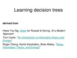
0. 1. X 2. X 3. 0. 1. 0. 1. 0. 1. 1. 0. Parikshit Gopalan MSR-Silicon Valley , IITB’00. Adam Tauman Kalai MSR-New England Adam R. Klivans UT Austin. Agnostically Learning Decision Trees. 1. 0. X 1. 0. 1. 1. 0. 0. 1. Computational Learning. Computational Learning.

Agnostically Learning Decision Trees
E N D
Presentation Transcript
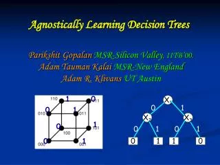
0 1 X2 X3 0 1 0 1 0 1 1 0 Parikshit GopalanMSR-Silicon Valley, IITB’00.Adam Tauman Kalai MSR-New EnglandAdam R. KlivansUT Austin Agnostically Learning Decision Trees 1 0 X1 0 1 1 0 0 1
Computational Learning f:{0,1}n! {0,1} x, f(x) Learning: Predict f from examples.
Valiant’s Model f:{0,1}n! {0,1} Halfspaces: + + + + + - + x, f(x) - + - - - + - - - - - - Assumption: f comes from a nice concept class.
0 1 X2 X3 0 1 0 1 0 1 1 0 Valiant’s Model f:{0,1}n! {0,1} Decision Trees: X1 x, f(x) Assumption: f comes from a nice concept class.
X1 0 1 X2 X3 0 1 0 1 0 1 1 0 The Agnostic Model [Kearns-Schapire-Sellie’94] f:{0,1}n! {0,1} Decision Trees: x, f(x) No assumptions about f. Learner should do as well as best decision tree.
X1 0 1 X2 X3 0 1 0 1 0 1 1 0 The Agnostic Model [Kearns-Schapire-Sellie’94] Decision Trees: x, f(x) No assumptions about f. Learner should do as well as best decision tree.
X1 0 1 X2 X3 0 1 0 1 0 1 1 0 Agnostic Model = Noisy Learning f:{0,1}n! {0,1} + = • Concept: Message • Truth table: Encoding • Function f: Received word. • Coding: Recover the Message. • Learning:Predict f.
Uniform Distribution Learning for Decision Trees • Noiseless Setting: • No queries:nlog n[Ehrenfeucht-Haussler’89]. • With queries:poly(n). [Kushilevitz-Mansour’91] Agnostic Setting: Polynomial time, uses queries. [G.-Kalai-Klivans’08] Reconstruction for sparse real polynomials in the l1 norm.
The Fourier Transform Method • Powerful tool for uniform distribution learning. • Introduced by Linial-Mansour-Nisan. • Small depth circuits[Linial-Mansour-Nisan’89] • DNFs[Jackson’95] • Decision trees[Kushilevitz-Mansour’94, O’Donnell-Servedio’06, G.-Kalai-Klivans’08] • Halfspaces, Intersections[Klivans-O’Donnell-Servedio’03, Kalai-Klivans-Mansour-Servedio’05] • Juntas[Mossel-O’Donnell-Servedio’03] • Parities[Feldman-G.-Khot-Ponnsuswami’06]
The Fourier Polynomial • Let f:{-1,1}n! {-1,1}. • Write f as a polynomial. • AND:½ + ½X1 + ½X2 - ½X1X2 • Parity:X1X2 • Parity of ½ [n]: (x) = i 2Xi • Write f(x) = c()(x) • c()2 =1. Standard Basis Function f Parities
The Fourier Polynomial • Let f:{-1,1}n! {-1,1}. • Write f as a polynomial. • AND:½ + ½X1 + ½X2 - ½X1X2 • Parity:X1X2 • Parity of ½ [n]: (x) = i 2Xi • Write f(x) = c()(x) • c()2 =1. c()2: Weight of .
Low Degree Functions • Sparse Functions: Most of the weight lies on small subsets. • Halfspaces, Small-depth circuits. • Low-degree algorithm. [Linial-Mansour-Nisan] • Finds the low-degree Fourier coefficients. Least Squares Regression: Find low-degree P minimizing Ex[ |P(x) – f(x)|2 ].
Sparse Functions • Sparse Functions: Most of the weight lies on a few subsets. • Decision trees. t leaves )O(t) subsets • Sparse Algorithm. • [Kushilevitz-Mansour’91] Sparse l2 Regression: Find t-sparse P minimizing Ex[ |P(x) – f(x)|2 ].
Sparse l2 Regression • Sparse Functions: Most of the weight lies on a few subsets. • Decision trees. t leaves )O(t) subsets • Sparse Algorithm. • [Kushilevitz-Mansour’91] Sparse l2 Regression: Find t-sparse P minimizing Ex[ |P(x) – f(x)|2 ]. Finding large coefficients: Hadamard decoding. [Kushilevitz-Mansour’91, Goldreich-Levin’89]
f:{-1,1}n! {-1,1} +1 -1 Agnostic Learning via l2 Regression?
X1 0 1 X2 X3 +1 0 1 0 1 0 1 1 0 -1 Agnostic Learning via l2 Regression?
+1 -1 Agnostic Learning via l2 Regression? Target f Best Tree • l2 Regression: Loss |P(x) –f(x)|2 • Pay 1 for indecision. • Pay 4 for a mistake. • l1 Regression: [KKMS’05] • Loss |P(x) –f(x)| • Pay 1 for indecision. • Pay 2 for a mistake.
+1 -1 Agnostic Learning via l1 Regression? • l2 Regression: Loss |P(x) –f(x)|2 • Pay 1 for indecision. • Pay 4 for a mistake. • l1 Regression: [KKMS’05] • Loss |P(x) –f(x)| • Pay 1 for indecision. • Pay 2 for a mistake.
+1 -1 Agnostic Learning via l1 Regression Target f Best Tree Thm [KKMS’05]:l1 Regression always gives a good predictor. l1 regression for low degree polynomials via Linear Programming.
Agnostically Learning Decision Trees Sparse l1 Regression: Find a t-sparse polynomial P minimizing Ex[ |P(x) – f(x)|]. • Why is this Harder: • l2 is basis independent, l1 is not. • Don’t know the support of P. • [G.-Kalai-Klivans]: Polynomial time algorithm for Sparse l1Regression.
The Gradient-Projection Method L1(P,Q) = |c() – d()| L2(P,Q) = [ (c() –d())2]1/2 f(x) P(x) = c() (x) Q(x) = d() (x) Variables:c()’s. Constraint: |c() | · t Minimize:Ex|P(x) – f(x)|
Gradient The Gradient-Projection Method Variables:c()’s. Constraint: |c() | · t Minimize:Ex|P(x) – f(x)|
Gradient The Gradient-Projection Method Projection Variables:c()’s. Constraint: |c() | · t Minimize:Ex|P(x) – f(x)|
+1 -1 The Gradient • g(x) = sgn[f(x) - P(x)] • P(x) := P(x) + g(x). f(x) P(x) Increase P(x) if low. Decrease P(x) if high.
Gradient The Gradient-Projection Method Variables:c()’s. Constraint: |c() | · t Minimize:Ex|P(x) – f(x)|
Gradient The Gradient-Projection Method Projection Variables:c()’s. Constraint: |c() | · t Minimize:Ex|P(x) – f(x)|
Projection onto the L1 ball Currently: |c()| > t Want:|c()| · t.
Projection onto the L1 ball Currently: |c()| > t Want:|c()| · t.
Projection onto the L1 ball • Below cutoff:Set to 0. • Above cutoff:Subtract.
Projection onto the L1 ball • Below cutoff:Set to 0. • Above cutoff:Subtract.
Analysis of Gradient-Projection [Zinkevich’03] • Progress measure:Squared L2 distance from optimum P*. Key Equation: |Pt – P*|2 - |Pt+1 – P*|2¸ 2 (L(Pt) – L(P*)) • Within of optimal in 1/2 iterations. • Good L2 approximation to Pt suffices. – 2 Progress made in this step. How suboptimal current soln is.
+1 -1 Gradient f(x) • g(x) = sgn[f(x) - P(x)]. P(x) Projection
+1 -1 The Gradient • g(x) = sgn[f(x) - P(x)]. f(x) P(x) • Compute sparse approximation g’ = KM(g). • Is g a good L2 approximation to g’? • No. Initially g = f. • L2(g,g’) can be as large 1.
Sparse l1 Regression Approximate Gradient Variables:c()’s. Constraint: |c() | · t Minimize:Ex|P(x) – f(x)|
Sparse l1 Regression Projection Compensates Variables:c()’s. Constraint: |c() | · t Minimize:Ex|P(x) – f(x)|
KM as l2 Approximation The KM Algorithm: Input:g:{-1,1}n! {-1,1}, and t. Output: A t-sparse polynomial g’ minimizing Ex [|g(x) – g’(x)|2] Run Time: poly(n,t).
KM as L1 Approximation The KM Algorithm: Input: A Boolean function g = c()(x). A error bound . Output: Approximation g’ = c’()(x) s.t |c() – c’()| · for all½ [n]. Run Time: poly(n,1/)
KM as L1 Approximation Only 1/2 • Identify coefficients larger than. • Estimate via sampling, set rest to 0.
KM as L1 Approximation • Identify coefficients larger than. • Estimate via sampling, set rest to 0.
Projection Preserves L1 Distance L1distance at most 2after projection. Both lines stop within of each other.
Projection Preserves L1 Distance L1distance at most 2after projection. Both lines stop within of each other. Else, Blue dominates Red.
Projection Preserves L1 Distance L1distance at most 2after projection. Projecting onto the L1 ball does not increase L1 distance.
Sparse l1 Regression • L1(P, P’) · 2 • L1(P, P’) · 2t • L2(P, P’)2· 4t P’ P Can take = 1/t2. Variables:c()’s. Constraint: |c() | · t Minimize:Ex|P(x) – f(x)|
Agnostically Learning Decision Trees Sparse L1 Regression: Find a sparse polynomial P minimizing Ex[ |P(x) – f(x)|]. • [G.-Kalai-Klivans’08]: • Can get within of optimum in poly(t,1/) iterations. • Algorithm for Sparsel1Regression. • First polynomial time algorithm for Agnostically Learning Sparse Polynomials.
l1 Regression from l2 Regression Functionf: D ! [-1,1],Orthonormal BasisB. Sparse l2 Regression: Find a t-sparse polynomial P minimizing Ex[ |P(x) – f(x)|2 ]. Sparse l1 Regression: Find a t-sparse polynomial P minimizing Ex[ |P(x) – f(x)|]. • [G.-Kalai-Klivans’08]:Given solution to l2 Regression, can solve l1 Regression.
Agnostically Learning DNFs? • Problem: Can we agnostically learn DNFs in polynomial time? (uniform dist. with queries) • Noiseless Setting: Jackson’s Harmonic Sieve. • Implies weak learner for depth-3 circuits. • Beyond current Fourier techniques. Thank You!