Decision Trees for Classification: SVM, GMM, and More
980 likes | 1.07k Vues
Explore the problem of classification through decision trees with SVM (Support Vector Machine), GMM (Gaussian Mixture Model), Bayes' Rule, learning algorithms, offline/online classifiers, test samples, and predictions. Learn about attribute assumptions, feature selection, and constructing decision trees. Understand the power of decision trees as intuitive tools for prediction and classification. Compare different classifiers and their properties using real-world examples and key requirements. Enhance your knowledge in machine learning and improve decision-making processes.

Decision Trees for Classification: SVM, GMM, and More
E N D
Presentation Transcript
Decision Trees Jianping Fan Dept of Computer Science UNC-Charlotte
The problem of Classification • Given a set of training samples and their attribute values (x) and labels (y), try to determine the labels y of new examples. • Classifier Training y = f(x) • Prediction y given x Test Samples Classifier Training Samples Learning Algorithms Predictions
The problem of Classification Training Samples Learning Algorithms Classifier offline online Test Samples Classifier Predictions
SVM & GMM (Bayes Rule) Training Samples Learning Algorithms Classifier y = f(x) offline online Test Samples x Classifier y = f(x) Predictions y
Gaussian Mixture Model (GMM) How to estimate the data distribution for a given dataset?
Bayes’ Rule: normalization Who is who in Bayes’ rule
Plane Bisect Closest Points wT x + b =-1 wT x + b =0 d c wT x + b =1
denotes +1 denotes -1 x+ x+ x- Large Margin Linear Classifier x2 • Formulation: Margin wT x + b = 1 such that wT x + b = 0 wT x + b = -1 n x1
denotes +1 denotes -1 wT x + b = 1 wT x + b = 0 wT x + b = -1 Large Margin Linear Classifier x2 • What if data is not linear separable? (noisy data, outliers, etc.) • Slack variables ξican be added to allow mis-classification of difficult or noisy data points x1
Large Margin Linear Classifier • Formulation: such that • Parameter C can be viewed as a way to control over-fitting.
Revisit of GMM & SVM • If features or attributes x are multi-dimensional, what kind of assumptions they have made for the features or attributes x? GMM: SVM: st. Assumption:
Example. ‘Play Tennis’ data Outlook, temperature, humidity, wind are not comparable directly!
SVM & GMM (Bayes Rule) Training Samples Learning Algorithms Classifier y = f(x) offline online Test Samples x Classifier y = f(x) Predictions y
SVM & GMM (Bayes Rule) cannot handle this case! Training Samples Learning Algorithms Classifier y = f(x) offline online Test Samples x Classifier y = f(x) Predictions y
Wish List: • Even these features or attributes x are not comparable directly, the decisions y they make could be comparable! • For different decisions y, we can use different features or attributes x! Classifier Training with Feature Selection!
Our Expectations Outlook sunny rainy overcast Humidity P Windy high normal yes no N P N P How to make this happen? Compare it with our wish list
Our Expectations Outlook sunny rainy overcast Humidity P Windy high normal yes no N P N P • Different nodes can select and use one single feature or attribute x • Use various paths to combine multiple features or attributes x How to select feature for each node? When we stop such path?
Decision Tree • What is a Decision Tree • Sample Decision Trees • How to Construct a Decision Tree • Problems with Decision Trees • Summary
Definition • Decision tree is a classifier in the form of a tree structure • Decision node: specifies a test on a single attribute or feature x • Leaf node: indicates the value of the target attribute (label) y • Arc/edge: split of one attribute (could be multiple partitions y or binary ones y) • Path: a disjunction of test to make the final decision (all attributes x could be used) • Decision trees classify instances or examples by starting at the root of the tree and moving through it until a leaf node.
Why decision tree? • Decision trees are powerful and popular tools for classification and prediction. • Decision trees represent rules, which can be understood by humans and used in knowledge system such as database. Compare these with our wish list
key requirements • Attribute-value description: object or case must be expressible in terms of a fixed collection of properties or attributes x (e.g., hot, mild, cold). • Predefined classes (target values y): the target function has discrete output values y (binary or multiclass) • Sufficient data: enough training cases should be provided to learn the model.
outlook sunny rainy yes company no big med no sailboat yes small big yes no An Example Data Set and Decision Tree
Classification outlook sunny rainy yes company no big med no sailboat yes small big yes no
DECISION TREE • An internal node is a test on an attribute. • A branch represents an outcome of the test, e.g., Color=red. • A leaf node represents a class label or class label distribution. • At each node, one attribute is chosen to split training examples into distinct classes as much as possible • A new case is classified by following a matching path to a leaf node. Each node uses one single feature to train one classifier!
SVM, GMM (Bayes Rule) & Decision Tree Training Samples Learning Algorithms Classifier y = f(x) offline online Test Samples x Classifier y = f(x) Predictions y One more weapon at hand now!
Decision Tree Construction • Top-Down Decision Tree Construction • Choosing the Splitting Attribute: Feature Selection • Information Gain and Gain Ratio: Classifier Training
Decision Tree Construction • Selecting the best-matching feature or attribute x for each node ---what kind of criteria can be used? • Training the node classifier y = f(x) under the selected feature x ---what kind of classifiers can be used?
Secondary Gleason Grade 1,2 3 4 5 No Yes PSA Level Stage 14.9 14.9 T1ab,T3 T1c,T2a,T2b,T2c No No Yes Primary Gleason Grade 2,3 4 No Yes Prostate cancer recurrence
Simple Tree Outlook sunny rainy overcast Humidity P Windy high normal yes no N P N P Decision Tree can select different attributes for different decisions!
Complicated Tree Given a data set, we could have multiple solutions! Temperature hot cold moderate Outlook Outlook Windy sunny rainy sunny rainy yes no overcast overcast P P Windy Windy P Humidity N Humidity yes no yes no high normal high normal N P P N Windy P Outlook P yes no sunny rainy overcast N P N P null
Attribute Selection Criteria • Main principle • Select attribute which partitions the learning set into subsets as “pure” as possible • Various measures of purity • Information-theoretic • Gini index • X2 • ReliefF • ... • Various improvements • probability estimates • normalization • binarization, subsetting
Information-Theoretic Approach • To classify an object, a certain information is needed • I, information • After we have learned the value of attribute A, we only need some remaining amount of information to classify the object • Ires, residual information • Gain • Gain(A) = I – Ires(A) • The most ‘informative’ attribute is the one that minimizes Ires, i.e., maximizes Gain
Entropy • The average amount of information I needed to classify an object is given by the entropy measure • For a two-class problem: entropy p(c1)
Residual Information • After applying attribute A, S is partitioned into subsets according to values v of A • Ires is equal to weighted sum of the amounts of information for the subsets
Triangles and Squares Data Set: A set of classified objects . . . . . .
Entropy • 5 triangles • 9 squares • class probabilities • entropy . . . . . .
. . . . . . . . red green yellow . . . . Entropyreductionbydata setpartitioning Color?
. . . . . . Entropija vrednosti atributa . . . . . . red Color? green yellow
. . . . . . Information Gain . . . . . . red Color? green yellow
Information Gain of The Attribute • Attributes • Gain(Color) = 0.246 • Gain(Outline) = 0.151 • Gain(Dot) = 0.048 • Heuristics: attribute with the highest gain is chosen • This heuristics is local (local minimization of impurity)
. . . . . . . . . . . . red Color? green yellow Gain(Outline) = 0.971 – 0 = 0.971 bits Gain(Dot) = 0.971 – 0.951 = 0.020 bits
. . . . . . . . . . . . . . Initial decision red Gain(Outline) = 0.971 – 0.951 = 0.020 bits Gain(Dot) = 0.971 – 0 = 0.971 bits Color? green yellow solid Outline? dashed Conditional decision
. . . . . . . . . . . . . . red . yes Dot? . Color? no green yellow solid Outline? dashed
Decision Tree . . . . . . Color red green yellow Dot square Outline yes no dashed solid triangle square triangle square
A Defect of Ires • Ires favors attributes with many values • Such attribute splits S to many subsets, and if these are small, they will tend to be pure anyway • One way to rectify this is through a corrected measure of information gain ratio.
Information Gain Ratio • I(A) is amount of information needed to determine the value of an attribute A • Information gain ratio
. . . . . . Information Gain Ratio . . . . . . red Color? green yellow