DECISION TREES
Understand the building process and algorithm behind decision trees, including top-down tree construction and bottom-up tree pruning. Learn about decision tree induction, attribute selection criteria, and information gain computation. Improve your decision-making skills with this comprehensive guide.

DECISION TREES
E N D
Presentation Transcript
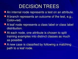
DECISION TREES • An internal node represents a test on an attribute. • A branch represents an outcome of the test, e.g., Color=red. • A leaf node represents a class label or class label distribution. • At each node, one attribute is chosen to split training examples into distinct classes as much as possible • A new case is classified by following a matching path to a leaf node.
Example Outlook sunny overcast rain humidity windy P high normal false true N P N P
Building Decision Tree • Top-down tree construction • At start, all training examples are at the root. • Partition the examples recursively by choosing one attribute each time. • Bottom-up tree pruning • Remove subtrees or branches, in a bottom-up manner, to improve the estimated accuracy on new cases. • Use of decision tree: Classifying an unknown sample • Test the attribute values of the sample against the decision tree
Output: A Decision Tree for “buys_computer” age? <=30 overcast >40 30..40 student? credit rating? yes no yes fair excellent no yes no yes
Algorithm for Decision Tree Induction • Basic algorithm (a greedy algorithm) • Tree is constructed in a top-down recursive divide-and-conquer manner • At start, all the training examples are at the root • Attributes are categorical • Examples are partitioned recursively based on selected attributes • Test attributes are selected on the basis of a heuristic or statistical measure (e.g., information gain) • Conditions for stopping partitioning • All samples for a given node belong to the same class • There are no remaining attributes for further partitioning – majority voting is employed for classifying the leaf • There are no samples left
Choosing the Splitting Attribute • At each node, available attributes are evaluated on the basis of separating the classes of the training examples. A Goodness function is used for this purpose. • Typical goodness functions: • information gain (ID3/C4.5) • information gain ratio • gini index
A criterion for attribute selection • Which is the best attribute? • The one which will result in the smallest tree • Heuristic: choose the attribute that produces the “purest” nodes • Popular impurity criterion: information gain • Information gain increases with the average purity of the subsets that an attribute produces • Strategy: choose attribute that results in greatest information gain
Information Gain (ID3/C4.5) • Select the attribute with the highest information gain • Assume there are two classes, P and N • Let the set of examples S contain p elements of class P and n elements of class N • The amount of information, needed to decide if an arbitrary example in S belongs to P or N is defined as
Information Gain in Decision Tree Induction • Assume that using attribute A a set S will be partitioned into sets {S1, S2 , …, Sv} • If Si contains piexamples of P and ni examples of N, the entropy, or the expected information needed to classify objects in all subtrees Si is • The encoding information that would be gained by branching on A
Class P: buys_computer = “yes” Class N: buys_computer = “no” I(p, n) = I(9, 5) =0.940 Compute the entropy for age: Hence Similarly Attribute Selection by Information Gain Computation
Example: attribute “Outlook” • “Outlook” = “Sunny”: • “Outlook” = “Overcast”: • “Outlook” = “Rainy”: • Expected information for attribute: Note: this is normally not defined.
Computing the information gain • Information gain: information before splitting – information after splitting • Information gain for attributes from weather data:
The final decision tree • Note: not all leaves need to be pure; sometimes identical instances have different classes Splitting stops when data can’t be split any further

