Modeling Excitonic Solar Cells: Insights from Dynamic Monte Carlo Simulations
This study, led by Alison Walker at the Department of Physics, explores the modeling of excitonic solar cells using Dynamic Monte Carlo simulations. It examines how modeling aids in understanding materials, self-organization, and device physics. Key topics include charge and energy transport, exciton behavior, and internal/external quantum efficiency. By analyzing varying morphologies and interfacial areas, this research addresses the complexities of exciton creation, hopping, dissociation, and recombination processes, revealing potential strategies for improving solar cell efficiency.

Modeling Excitonic Solar Cells: Insights from Dynamic Monte Carlo Simulations
E N D
Presentation Transcript
Modelling excitonic solar cells Alison Walker Department of Physics
How can modelling help? • Materials • Patterning, Self-organisation, Fabrication • Device Physics • Characterization
Outline • Dynamic Monte Carlo Simulation • Energy transport • Charge transport
Excitons generated throughout Electrons confined to green regions Holes confined to red regions P K Watkins, A B Walker, G L B Verschoor Nano Letts5, 1814 (2005)
Disordered morphology (a) Interfacial area 3106 nm2 (b) Interfacial area 1106 nm2 (c) Interfacial area 0.2106 nm2
Modelled Morphology • Hopping sites on a cubic latticewith lattice parameter a = 3 nm • Sites are either electron transporting polymer (e)or hole transporting polymer (h)
Ising Model • Ising energy for site i isi= -½J [(si, sj) – 1] • Summation over 1st and 2nd nearest neighbours • Spin at site isi= 1 for e site, 0 for h site • Exchange energy J = 1 • Chose neighbouring pair of sites l, m and findenergy difference = l- m • Spins swopped with probability
Internal quantum efficiency IQE IQEmeasures exciton harvesting efficiency Exciton dissociation efficiency e= no of dissociated excitons no of absorbed photons Charge transport efficiency c= no of electrons exiting device no of dissociated excitons Internal quantum efficiency IQE= no of electrons exiting device = e c no of absorbed photons NB Assume all charges reaching electrodes exit device
External quantum efficiency EQE For illumination with spectral density S() JSC = qd EQES() where external quantum efficiency EQE = no of electrons flowing in external circuit no of photons incident on cell = AIQE photon absorption efficiency A = no of absorbed photons no of photons incident on cell internal quantum efficiency IQE = no of electrons flowing in external circuit no of absorbed photons
Possible reactions • Exciton creation on either e or h site • Exciton hopping between sites of same type • Exciton dissociation at interface between e and h sites • Exciton recombination • Electron(hole) hopping between e(h) sites • Electron(hole) extraction • Charge recombination
Generation of morphologies with varying interfacial area • Start with a fine scale of interpenetration, corresponding to a large interfacial area • As time goes on, free energy from Ising model is lowered, favouring sites with neighbours that are the same type • Hence interfacial area decreases • Systems with different interfacial areas are morphologies at varying stages of evolution
Challenges • Several interacting particle species • Many possible interactions:GenerationHoppingRecombinationExtraction • Wide variation in time scales • Two site types
Why use Monte Carlo ? • Do not have (or want) detailed information about particle trajectories on atomic length scales nor reaction rates • Thus can only give probabilities for reaction times • These can be obtained by solving the Master equation but this is computationally costly for 3D systems
Dynamical Monte Carlo Model • Many different methods • These can all be shown to solve the Master Equation (Jansen*) • First Reaction Method has been used to simulate electrons only in dye-sensitized solar cells *A P J Jansen Phys Rev B 69, 035414 (2004) A P J Jansen http://ar.Xiv.org/, paper no. cond-matt/0303028
(W P- W P) dP = dt Master equation ,are configurationsP, Pare their probabilities Ware the transition rates
Simple derivation of Poisson Distribution Consider a reaction with a transition rate k. Probability that a reaction occurs in time intervalt t + dt dp = (Probability reaction does not occur before t) (Probability reaction occurs in dt) = - p(t) k dt Hence probability distribution P(t) of times at which reaction occurs normalised such that P(t)dt = 1 is the Poisson distribution P(t) = kexp(-kt) R Hockney, J W Eastwood Computer simulation using particles IoP Publishing, Bristol, 1988
Selecting waiting times Integrating dc= dp= P(t) dt gives cumulative probability c(t) = 0t P(t)dt The reaction has not occurred at t = 0 but will occur some time, so c(0) = 0 c 1=c() If the value of c is set equal to a random number r chosen from a uniform distribution in the range 0 r 1, the probability of selecting a value in the range c c + dc isdc Hence r = c(t) = 0t P(t)dt
eg for a distribution peaked at x0, most values of r will give values of x close to x0 1 r 0 x x0 c f 1 r 0 x0 F x For Poisson distribution, P t t t0
t= -1 ln(1-r1) = -1 ln(r2) k k To select times with Poisson distribution from random numbers ri distributed uniformly between 0 and 1, use r1 = 0t kexp(-kt)dt Hence
i = -1ln(r) wi First Reaction Method • Each reaction i with rate wihas a waiting time from a uniformly distributed random number r • Listof reactions created in order of increasing i • First reaction in list takes place if enabled • List then updated
Top reaction enabled? Create a queue of reactions i and associated waiting times i. Set simulation timet = 0. Select reaction at top of queue Flow Chart Remove from queue No Yes Do top reaction Remove this reaction from queue Set t = t + top Seti =i - top Add enabled reactions
Simulation details • Hops allowed to the 122 neighbours within 9 nm cutoff distance • Exclusion principle applies ie hops disallowed to occupied sites • Periodic boundary conditions in x and y • Site energies Ei are all zero for excitons • For charge transport, Ei include(i) Coulomb interactions(ii) external field due to built-in potential and external voltage
Electron(hole) hopping between e(h) sites wij = w0exp[-2Rij]exp[-(Ej – Ei)/(kBT)] if Ej > Eiw0exp[-2Rij] if Ej < Eiw0 = [6kBT/(qa2)]exp[-2a]e = h = 1.10-3 cm2/(Vs) = 2 nm-1 • Electron(hole) recombination ratewce = 100 s-1allows peak IQE to exceed 50% for idealisedmorphology • Electron(hole) extractionwce = if electron next to anode/hole next to cathode wce = 0 otherwise
Reaction rates • Exciton creation on either e or h siteS = 2.4102 nm-2s-1 • Exciton hopping between sites of same typewij = we(R0/Rij)6 weR06 = 0.3 nm6s-1 gives diffusion length of 5nm • Exciton dissociation at interface between e and h siteswed = if exciton on an interface sitewed = 0 otherwise
Disordered morphology (a) Interfacial area 3106 nm2 (b) Interfacial area 1106 nm2 (c) Interfacial area 0.2106 nm2
excitons more likely to find an interface before recombining • thus exciton dissociation efficiency increases • charges follow more tortuous routes to get to electrodes • charge densities are higher • charge recombination greater • thus charge transport efficiency decreases • Net effect is a peak in the internal quantum efficiency At large interfacial area ie small scale phase separation:
Sensitivity of IQE to input parameters • As the exciton generation rate increases,IQE decreases at all interfacial areas due to enhanced charge recombination • For larger external biases, the peak IQE increases and shifts to larger interfacial areas • Similar changes to (b) seen for larger charge mobilities and if charge mobilities differ
Ordered morphology Achievable with diblock copolymers
As for disordered morphologies, see a peak in IQE, here at a width of 15 nm • Maximum IQE is larger by a factor of 1.5 than for disordered morphologies • Peak is sharper since at large interfacial areas, excitons less likely to find an interface and the charges are confined to narrow regions so there is a large recombination probability.
Gyroids • Continuous charge transport pathways, no disconnected or ‘cul-de-sac’ features • Free from islands • A practical way of achieving a similar efficiency to the rods?
Recombination Geminate recombination Unexpected difference between rod structures and the others. • Bimolecular recombination • Novel structures show little advantage over blends (even at 5 suns). Islands and disconnected pathways not responsible for inefficiency as previously thought • Rod structures significantly better, even at small feature sizes • Short, direct pathways to electrodes • Can keep charges entirely isolated
Why? E • Most time is spent tracking at the interface. • A polymer with a range of interface angles is far less efficient than a vertical structure.
Feature size dependence of fill factor, shift in optimum feature size when examining complete J-V performance. • Islands shift the perceived optimum feature size. • New morphologies not as efficient as hoped, despite absence of islands and disconnected pathways. • Morphology can still inhibit geminate separation at large feature sizes. • Rods have noticeably lower geminate and bimolecular recombination, but for different reasons. • Angle of interface is critical, morphologies with a range of angles less efficient than vertical structures.
Dynamical Monte CarloSummary Dynamical Monte Carlo methods are a useful way of modelling polymer blend organic solar cells because (i) they are easy to implement, (ii) they can handle interacting particles (iii) they can be used with widely varying time scales
Energy transport Stavros Athanasopoulos, David Beljonne, Evgenia Emilianova University of Mons-Hainaut Luca Muccioli, Claudio Zannoni University of Bologna
electronic properties Chemical structure Physical morphology
Experimental background • Polyphenylenes eg PFO used for blue emissive layers in blue OLEDs but emission maxima close to violet • Polyindenofluorenes intermediate between PFO and LPPP show purer blue emission • The solid state luminescence output has been related to the microscopic morphology
Spectroscopy on end-capped polymers Solution Solid PL intensity l (nm) Indenofluorene chromophores Perylene end-caps
Transfer rates from chromophore to perylene are much faster than those between chromophores • Different spectra are observed for the polymer in solution, and as a film
Morphology P3HT- crystalline, high mobility (~0.1 cm2/Vs) Disorder could occur parallel to plane of substrate
Electron micrograph of PF2/6: Liquid-crystalline state lamellae separated by disordered regions; molecules inside lamellaeseparate according tolengths Ordered regions also seenin PIF copolymers
Numbers of chromophores per chain, and lengths of individual chromophores are assigned specified distributions:
Key Features of our Model • Exciton diffusion takes place within a realistic morphology consisting of a 3D array of PIF chains • Excitons hop between chromophores • Averaging over many exciton trajectories, properties such as diffusion length, ratio of numbers of intrachain to interchain hops, spectra etc are explored
Quantum Chemical Calculation of Hopping Rates • Mons provide rates of exciton transfer between chromophores • They use quantum chemical calculations employing the distributed monopole method • This takes into account the shape of donor and acceptor chromophores in calculating the electronic coupling Vda • The hopping rate from donor to acceptor is Electronic coupling Overlap factor
Trajectories of individual particles (note periodic boundary conditions) are averaged to obtain quantities of interest