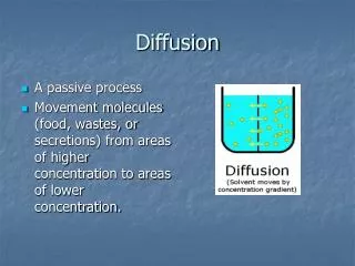
Chapter 5 Diffusion
Chapter 5 Diffusion. Diffusion :. During production and application, the chemical composition of engineering materials is often changed as a result of the movement of atoms, or solid-state diffusion.

Chapter 5 Diffusion
E N D
Presentation Transcript
Diffusion : During production and application, the chemical composition of engineering materials is often changed as a result of the movement of atoms, or solid-state diffusion. Diffusion makes atoms 1). redistribute, 2). move in from out side, 3). move out of the materials. Therefore, understanding the nature of the movement of atoms within the material can be critically important both in producing the material and in using it successfully within an engineering design. Vacancy, which is produced by thermal vibration, helps diffusion, therefore, the diffusion process is also affected by the thermal vibration. The rate of diffusion increases exponentially with temperature. Mathematics of diffusion allows a calculation of the variation of the chemical composition within the materials at a given temperature and given heating time. An important example is the carburization of steels, in which the surface is hardened by the diffusion of carbon atoms from a carbon-rich environment. Phase transformation and heat treatment are controlled by diffusion process.
5.1 Thermally Activated Processes Diffusion is one of the thermally activated processes and expressed by the Arrhenius type equation; Rate = C e-Q/RT or, ln(rate) = ln C - (5.1) Figure 5.1Typical Arrhenius plot of data compared with Equation 5.2. The slope equals −Q/R, and the intercept (at 1/T = 0) is ln C. (5.2) (See the text for all the parameters.) The eqn. (5.2) indicates that if the ln(R) is plotted against the 1/T, then there will be a strait line whose slope is equal to –Q/R. From this slope, one can get the activation energy of the process or the mechanism of the diffusion. One needs to have at least three temperature tests to get a straight line for the reliable slope or Q value and C value. Extrapolation of the plot to 1/T=0 (or T=∞) gives an intercept equal to lnC
In the previous eqn. (5.1), the unit of Q is “ Energy per Mol”. It is possible to write this eqn. by dividing both Q and R by Avogadro’s number(NAv), gives as follow; overcome by thermal activation Figure 5.2Process path showing how an atom must overcome an activation energy, q, to move from one stable position to a similar adjacent position. rate = Ce-q/kT (5.3) ①. q(= Q/NAv) : activation E. per atomic scale unit (atom, electron, and ion), ②. k(=R/NAv) : Boltzmann’s const. ( 13.8 X 10⁻²⁴J/K) Eqn. (5.3) provides for an interesting comparison with the high-energy end of the Maxwell-Boltzmann distribution of molecular energies in gases, p∝e∆E/kT(5.4), where, p is the probability of finding a molecule at an energy ∆E greater than the average energy characteristic of a particular temperature, T. This eqn. (5.4) is originally developed for gases, it applies to solid as well. As T increases, a larger number of atoms is available to overcome a given energy barrier, q.
Activation energy → activation mechanism As it is shown in Figure 5.2, we can understand the physical meaning of the activation energy, which can explain the activation mechanism. In practice, particular values of activation energy will be found to be characteristic of process mechanisms. In each case, it is useful to remember that various possible mechanisms may be occurring simultaneously within the material, and each mechanism has a characteristic activation energy. The fact that one activation energy is representative of the experimental data means simply that a single mechanism is dominant. If the process involves several sequential steps, the slowest step will be the rate-limiting step. Then this activation energy of the rate-limiting step will be the activation energy for the overall process.
Increase in ∆E Position 2 Most unstable position Figure 5.3Simple mechanical analog of the process path of Figure 5.2. The box must overcome an increase in potential energy, ΔE, in order to move from one stable position to another. Emax Center of gravity Emin Position 1 Position 3 This figure shows a simple mechanical model of activation energy in which a box is moved from one stable position to another by going through an increase in potential energy, ∆E, analogous to the q in Figure 5.2. of atomic scale.
Examples and Practice Problems : Students are asked to review the “Example” of 5.1 and solve the “Practice Problem” of 5.1 in the text.
5.2 Thermal Production of Point Defects Point defects are generated by the Thermal vibration (periodic oscillation) of atoms in the crystal structure. As T↑, the vibration ↑, → point defects (mainly vacancies in this section) ↑. At a given T. the avg. thermal E. is fixed. But thermal E. of the individual atoms varies over a wide range, as indicated Maxwell-Boltzmann distribution. At a given T., a certain fraction of atoms have sufficient thermal E. to produce point defects. Therefore, the fraction increases exponentially with absolute T by the Maxwell-Boltzmann distribution, as shown below; ndefects =Ce-(Edefect)/kT (5.5) (For the parameters, see the text P. 142.) nsites The defect formation energy value, Edefect, is different for the different defect.
∆L/L:expansion of material, which includes increased vacancy conc. ∆α/α: lattice expansion only, tested by x-ray diffraction technique. Figure 5.4(a) The overall thermal expansion (ΔL/L) of aluminum is measurably greater than the lattice parameter expansion (Δa/a) at high temperatures because vacancies are produced by thermal agitation. (b) A semilog (Arrhenius-type) plot of ln (vacancy concentration) versus 1/T based on the data of part (a). The slope of the plot (−Ev/k) indicates that 0.76 eV of energy is required to create a single vacancy in the aluminum crystal structure. (From P. G. Shewmon, Diffusion in Solids, McGraw-Hill Book Company, New York, 1963.) As T ↑, vacancy ↑→∴ the overall expansion of the crystal is more than that of lattice expansion and this trend is even more significant with increasing temperature. This indicates that as T ↑, the vacancy concentration is increased more. From this experiment, it is known that vacancy generation is thermally activated process and so expressed by the Arrhenius type equation. Aluminum Ev=0.76 eV nv ln =lnC-(Ev/kT) nsites
Examples and Practice Problems : Students are asked to review the “Example” of 5.2 and solve the “Practice Problem” of 5.2 in the text.
5.3 Point Defects and Solid-State Diffusion Figure 5.5Atomic migration occurs by a mechanism of vacancy migration. Note that the overall direction of material flow (the atom) is opposite to the direction of vacancy flow. With the help of thermal vibration, at sufficiently high temperature, atoms and molecules can be quite mobile to move around through the sites of vacancies i.e., selfdiffusion is taking place. Diffusion = vacancy migration
Figure 5.6Diffusion by an interstitialcy mechanism illustrating the random-walknature of atomic migration. (Random–walkis also done by the vacancy mechanism.) Random-walk itself does not make any directional motion of the element, even though the element has moved quite a long distance.
pure pure This atomic scale illustration shows that diffusion is taking place by vacancy mechanism for two similar size atoms. t = 0 Figure 5.7The interdiffusion of materials A and B. Although any given A or B atom is equally likely to “walk” in any random direction (see Figure 5.6), the concentration gradients of the two materials can result in a net flow of A atoms into the B material, and vice versa. (From W. D. Kingery, H. K. Bowen, and D. R. Uhlmann, Introduction to Ceramics, 2nd ed., John Wiley & Sons, Inc., New York, 1976.) As time passes Even though atom A and atom B are moving by vacancy mechanism random walk, because of the concentration gradient of A and B, interdiffusion is taking place to make the composition uniform. Complete of A and B
Concentration gradient profile Figure 5.8The interdiffusion of materials on an atomic scale was illustrated in Figure 5.7. This interdiffusion of copper and nickel is a comparable example on the microscopic scale.
Figure 5.9Geometry of Fick’s first law (Equation 5.8). Graphical illustration for the concentration change by interdiffusion. Fick’s 1st law : This law shows the concentration gradient at a given position under a given temperature (D=function of T).
CA = cont. Change in CA at B side with time. Fick’s second law Figure 5.10Solution to Fick’s second law (Equation 5.10) for the case of a semi-infinite solid, constant surfaceconcentration of the diffusing species cs , initial bulk concentration c0, and a constant diffusion coefficient, D (or const. T). ∂Cx ∂Cx ∂ ) ( D (5.9) = ∂t ∂x ∂x B side Aside Since D is independent of C, the above eqn. is rewritten as; (could be gas) 2 ∂Cx ∂Cx (5.10) ( ) = D ∂t ∂x 2 Carburization is a good example of this case! 0
Non-steady state diffusion ( Fick’s 2nd law) Consider a region of solid where concentration varies as (a) with distance. Flux (proportional to concentration gradient) will change as (b) For small distance Δx, J1> J2 . There will be concentration of solute atom in this region must increase. `
(See Table 5.1 for the values of “erf”) The solution to the differential eqn. of (5.10) ; Cx – C0 x = 1- erf ( ) (5.11) Cs – C0 Figure 5.11Master plot summarizing all of the diffusion results of Figure 5.10 on a single curve. 2√Dt This plot permits rapid calculation of the time necessary for relative saturation of the solid as a function of x, D and t.
Figure 5.12Saturation curves similar to that shown in Figure 5.11 for various geometries. The parameter cm is the average concentration of diffusing species within the sample. Again, the surface concentration, cs , and diffusion coefficient, D, are assumed to be constant. (From W. D. Kingery, H. K. Bowen, and D. R. Uhlmann, Introduction toCeramics, 2nd ed., John Wiley & Sons, Inc., New York, 1976.) skip
In the previous discussions, it was assumed that the diffusivity, D, was constant, or temperature was kept constant. D of Carbon in α-Fe with T. Figure 5.13Arrhenius plot of the diffusivity of carbon in α-iron over a range of temperatures. Note also related Figures 4.4 and 5.6 and other metallic diffusion data in Figure 5.14. (A good example of interstitialcy mechanism.) However, as it has been seen that the higher the temperature, the more the vacancy concentration. This means that the diffusivity may be influenced by the temperature and it is known that diffusivity data are well explained by the Arrhenius equation as follow ; D = D0 e –q /kT(5.12) where, D0 is preexponential const. and q is the defect migration activation energy for interstitial diffusion. For vacancy diffusion mechanism, q is the combination of formation and migration activation energy.
It is more common to tabulate diffusivity data in terms of molar quantities, i.e., with an activation energy, Q, per mole of diffusing species ; D = D0 e-Q/RT Figure 5.14Arrhenius plot of diffusivity data for a number of metallic systems. (From L. H. Van Vlack, Elements of Materials Science and Engineering, 4th ed., Addison-Wesley Publishing Co., Inc., Reading, MA, 1980.) C in fcc Fe D = D0 e-Q/RT(5.13) Comparison of C diffusion in Fe; Dbcc > Dfcc , but Qbcc< Qfcc. The larger Q, the smaller D. (Explain in terms of crystal structural character.) Cu in Al Fe diffusion in Fe (self diffusion) is similar to that of C in Fe diffusion.
Figure 5.15Arrhenius plot of diffusivity data for a number of nonmetallic systems. (From P. Kofstad, Nonstoichiometry, Diffusion, and Electrical Conductivity in Binary Metal Oxides, John Wiley & Sons, Inc., NY, 1972; and S. M. Hu in Atomic Diffusion in Semiconductors, D. Shaw, Ed., Plenum Press, New York, 1973.)
Examples and Practice Problems : Students are asked to review the “Example” of 5.3 ~5.6 and solve the “Practice Problem” of 5.3 ~ 5.6 in the text.
5.4 Steady-State Diffusion As time passes, a given concentration, Cg , is increased to be reached up to the value of the dotted red line, steady state conc. Figure 5.16Solution to Fick’s second law (Equation 5.10) for the case of a solid of thickness x0, constant surface concentrations of the diffusing species ch and cl , and a constant diffusion coefficient D. For long times (e.g., t3), the linear concentration profile is an example of steady-state diffusion. At the steady state, the concentration gradient in Fick’s 1st law can be written as; Cg Ch - Cl Ch - Cl ∆c ∂c As time increased = - = = (5.14) x0 ∂x ∆x 0 – x0 This Fig. is the case when the metal with thickness x0 is located in the environment of constant gas concentration of Ch in one side and Cl in the other side. (See Fig. 5.17) Since, this x0 is facing with Cl , it can not be increased.
Figure 5.17Schematic of sample configurations in gas environments that lead, after a long time, to the diffusionprofiles representative of (a) nonsteady state diffusion (Figure 5.10) and (b) steady-state diffusion (Figure 5.16).
Examples and Practice Problems : Students are asked to review the “Example” of 5.7 and solve the “Practice Problem” of 5.7 in the text.
5.5 Alternate Diffusion Paths There may be several different diffusion paths such as; 1). Volume diffusion or bulk diffusion, 2). Grain boundary diffusion, 3). Dislocation pipe diffusion, 4). Surface diffusion. Figure 5.18Self-diffusion coefficients for silver depend on the diffusion path. In general, diffusivity is greater through less-restrictive structural regions. (From J. H. Brophy, R. M. Rose, and J. Wulff, The Structure and Properties of Materials, Vol. 2: Thermodynamics of Structure, John Wiley & Sons, Inc., New York, 1964.) Since the slope of the plots implies, the activation energy of diffusion, the steeper the slope, the larger the Qdiff , so slower diffusion rate with smaller D values.. Qvol > QGB >Qsur→ Dvol<DGB<Dsur
Figure 5.19Schematic illustration of how a coating of impurity B can penetrate more deeply into grain boundaries and even further along a free surface of polycrystalline A, consistent with the relative values of diffusion coefficients (Dvolume < Dgrain boundary < Dsurface). At the beginning, diffusion is taking place through “surface” only with fast diffusion rate. As time passes, bulk diffusion is predominant and is slower. But the boundary diffusion is taking over the volume diffusion.
Examples and Practice Problems : Students are asked to review the “Example” of 5.8 and solve the “Practice Problem” of 5.8 in the text.