Learning Objectives

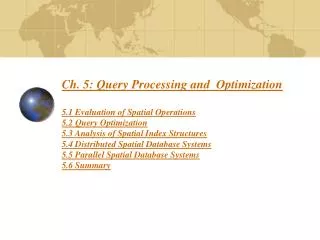
Chap4: Spatial Storage and Indexing4.1 Storage:Disk and Files4.2 Spatial Indexing4.3 Trends4.4 Summary

Learning Objectives • Learning Objectives (LO) • LO1: Understand concept of a physical data model • What is a physical data model? • Why learn about physical data models? • LO2 : Learn how to efficiently use storage devices • LO3: Learn how to structure data files • LO4: Learn how to use auxiliary data-structures • LO5: Learn about technology trends in physical data model • Focus on concepts not procedures! • Mapping Sections to learning objectives • LO2, LO3 - 4.1 • LO4 - 4.2 • LO5 - 4.3

Physical model in 3 level design? • Recall 3 levels of database design • Conceptual model: high level abstract description • Logical model: description of a concrete realization • Physical model: implementation using basic components • Analogy with vehicles • Conceptual model: mechanisms to move, turn, stop, ... • Logical models: • Car: accelerator pedal, steering wheel, brake pedal, … • Bicycle: pedal forward to move, turn handle, pull brakes on handle • Physical models : • Car: engine, transmission, master cylinder, break lines, brake pads, … • Bicycle: chain from pedal to wheels, gears, wire from handle to brake pads • We now go, so to speak, “under the hood”

What is a physical data model? • What is a physical data model of a database? • Concepts to implement logical data model • Using current components, e.g. computer hardware, operating systems • In an efficient and fault-tolerant manner • Why learn physical data model concepts? • To be able to choose between DBMS brand names • Some brand names do not have spatial indices! • To be able to use DBMS facilities for performance tuning • For example, If a query is running slow, • one may create an index to speed it up • For example, if loading of a large number of tuples takes for ever • one may drop indices on the table before the inserts • and recreate index after inserts are done!

Concepts in a physical data model • Database concepts • Conceptual data model - entity, (multi-valued) attributes, relationship, … • Logical model - relations, atomic attributes, primary and foreign keys • Physical model - secondary storage hardware, file structures, indices, … • Examples of physical model concepts from relational DBMS • Secondary storage hardware: Disk drives • File structures - sorted • Auxiliary search structure - • search trees (hierarchical collections of one-dimensional ranges)

An interesting fact about physical data model • Physical data model design is a trade-off between • Efficiently support a small set of basic operations of a few data types • Simplicity of overall system • Each DBMS physical model • Choose a few physical DM techniques • Choice depends chosen sets of operations and data types • Relational DBMS physical model • Data types: numbers, strings, date, currency • one-dimensional, totally ordered • Operations: • search on one-dimensional totally order data types • insert, delete, ...

Physical data model for SDBMS • Is relational DBMS physical data model suitable for spatial data? • Relational DBMS has simple values like numbers • Sorting, search trees are efficient for numbers • These concepts are not natural for Spatial data (e.g. points in a plane) • Reusing relational physical data model concepts • Space filling curves define a total order for points • This total order helps in using ordered files, search trees • But may lead to computational inefficiency! • New spatial techniques • Spatial indices, e.g. grids, hiearchical collection of rectangles • Provide better computational performance

Common assumptions for SDBMS physical model • Spatial data • Dimensionality of space is low, e.g. 2 or 3 • Data types: OGIS data types • Approximations for extended objects (e.g. linestrings, polygons) • Minimum Orthogonal Bounding Rectangle (MOBR or MBR) • MBR(O) is the smallest axis-parallel rectangle enclosing an object O • Supports filter and refine processing of queries • Spatial operations • OGIS operations, e.g. topological, spatial analysis • Many topological operations are approximated by “Overlap” • Common spatial queries - listed in next slide

Common Spatial Queries and Operations • Physical model provides simpler operations needed by spatial queries! • Common Queries • Point query: Find all rectangles containing a given point. • Range query: Find all objects within a query rectangle. • Nearest neighbor: Find the point closest to a query point. • Intersection query: Find all the rectangles intersecting a query rectangle. • Common operations across spatial queries • find : retrieve records satisfying a condition on attribute(s) • findnext : retrieve next record in a dataset with total order • after the last one retrieved via previous find or findnext • Nearest neighbor of a given object in a spatial dataset

Scope of discussion • Learn basic concepts in physical data model of SDBMS • Review related concepts from physical DM of relational DBMS • Reusing relational physical data model concepts • Space filling curves define a total order for points • This total order helps in using ordered files, search trees • But may lead to computational inefficiency! • New techniques • Spatial indices, e.g. grids, hiearchical collection of rectangles • Provide better computational performance

Learning Objectives • Learning Objectives (LO) • LO1: Understand concept of a physical data model • LO2 : Learn how to efficiently use storage devices • Concepts in Storage Hierarchy • Characteristics of secondary storage • Using secondary storage efficiently • LO3: Learn how to structure data files • LO4: Learn how to use auxiliary data-structures • LO5: Learn about technology trends in physical data model • Mapping Sections to learning objectives • LO2, LO3 - 4.1 (4.1.1) • LO4 - 4.2 • LO5 - 4.3

Storage Hierarchy in Computers • Computers have several components • Central Processing Unit (CPU) • Input, output devices, e.g. mouse, keyword, monitors, printers • Communication mechanisms, e.g. internal bus, network card, modem • Storage Hierarchy • Types of storage Devices • Main memories - fast but content is lost when power is off • Secondary storage - slower, retains content without power • Tertiary storage - very slow, retains content, very large capacity • DBMS usually manage data • on secondary storage, e.g. disks • Use main memory to improve performance • User tertiary storage (e.g. tapes) for backup, archival etc.

Secondary Storage Hardware: Disk Drives • Disk concepts • Circular platters with magnetic storage medium • Multiple platters are mounted on a spindle • Platters are divided into concentric tracks • A cylinder is a collection of tracks across platters with common radium • Tracks are divided into sectors • A sector size may a few kilo-Bytes • Disk drive concepts • Disk heads to read and write • There is disk head for each platter (recording surface) • A head assembly moves all the heads together in radial direction • Spindle rotates at a high speed, e.g. thousands revolution per minute • Accessing a sector has three major steps: • Seek: Move head assembly to relevant track • Latency: Wait for spindle to rotate relevant sector under disk head • Transfer: Read or write the sector • Other steps involve communication between disk controller and CPU

Using Disk Hardware Efficiently • Disk access cost are affected by • Placement ofdata one the disk • Fact than seek cost > latency cost > transfer (See Table 4.2, pp. 86) • A few common observations follow • Size of sectors • Larger sector provide faster transfer of large data sets • But waste storage space inside sectors for small data sets • Placement of most frequently accessed data items • On middle tracks rather than innermost or outermost tracks • Reason: minimize average seek time • Placement of items in a large data set requiring many sectors • Choose sectors from a single cylinder • Reason: Minimize seek cost in scanning the entire data set.

Software view of Disks: Fields, Records and File • Views of secondary storage (e.g. disks) • Hardware views - discussed in last few slides • Software views - Data on disks is organized into fields, records, files • Concepts • Field presents a property or attribute of a relation or an entity • Records represent a row in a relational table • Collection of fields for attributes in relational schema of the table • Files are collections of records • Homogeneous collection of records may represent a relation • Heterogeneous collections may be a union of related relations.

Mapping Records and files to Disk Fig 4.1 • Records • Often smaller than a sector • Many records in a sector • Files with many records • Many sectors per file • File system • Collection of files • Organized into directories • Mapping tables to disk • Figure 4.1 • City table takes 2 sectors • Others take 1 sector each

4.1.2 Buffer Management • Motivation • Accessing a sector on disk is much slower than accessing main memory • Idea: Keep repeatedly accessed data in main memory buffers • To improve the completion time of queries • Reducing load on disk drive • BufferManagersoftware module decides • Which sectors stay in main memory buffers? • Which sector is moved out if we run out of memory buffer space? • When to pre-fetch sector before access request from users? • These decision are based on the disk access patterns of queries!

Learning Objectives • Learning Objectives (LO) • LO1: Understand concept of a physical data model • LO2 : Learn how to efficiently use storage devices • LO3: Learn how to structure data files • What is a file structure? Why structure files? • What are common structures for spatial datafile? • LO4: Learn how to use auxiliary data-structures • LO5: Learn about technology trends in physical data model • Mapping Sections to learning objectives • LO2, LO3 - 4.1 • LO4 - 4.2 • LO5 - 4.3

4.1.4 File Structures • What is a file structure? • A method of organizing records in a file • For efficient implementation of common file operations on disks • Example: ordered files • Measure of efficiency • I/O cost: Number of disk sectors retrieved from secondary storage • CPU cost: Number of CPU instruction used • See Table 4.1 for relative importance of cost components • Total cost = sum of I/O cost and CPU cost

4.1.4 File Structures - selected file operations • Common file operations • Find: key value --> record matching key values • Findnext --> Return next record after find if records were sorted • Insert --> Add a new record to file without changing file-structure • Nearest neighbor of a object in a spatial dataset • Examples using Figure 4.1, pp. 88 • find(Name = Canada) on Country table returns recird about Canada • findnext() on Country table returns record about Cuba • since Cuba is next value after Canada in sorted order of Name • insert(record about Panama) into Country table • adds a new record • location of record in Country file depends on file-structure • nearest neighbor Argentina in country table is Brazil

4.1.4 Common File Structures • Common file structures • Heap or unordered or unstructured • Ordered • Hashed • Clustered • Descriptions follow • Basic Comparison of Common File Structures • Heap file is efficient for inserts and used for logfiles • But find, findnext, etc. are very slow • Hashed files are efficient for find, insert, delete etc. • But findext is very slow • Orderd file oranization are very fast for findnext • and pretty competent for find, insert, etc.

4.1.4 File Structures: Heap, Ordered • Heap • Records are in no particular order (Example: Figure 4.1) • insert can simple add record to the last sector • find, findnext, nearest neighbor scan the entire files • Ordered • Records are sorted by a selected field (Example Fig. 4.3 below) • findnext can simply pick up physically next record • find, insert, delete may use binary search, is is very efficient • nearest neighbor processed as a range query (seepp. 95 for details) Figure 4.3

File Structure : Hash • Components of a Hash file structure (Fig. 4.2) • A set of buckets (sectors) • Hash function : key value --> bucket • Hash directory: bucket --> sector • Operations • find, insert, delete are fast • compute hash function • lookup directiry • fetch relevant sector • findnext, nearest neighbor are slow • no order among records Fig 4.2

4.1.5 Spatial File Structures: Clustering • Motivation: • Ordered files are not natural for spatial data • Clustering records in sector by space filling curve is an alternative • In general, clustering groups records • accessed by common queries • into common disk sectors • to reduce I/O costs for selected queries • Clustering using Space filling curves • Z-curve • Hilbert-curve • Details on following 3 slides

Z-Curve • What is a Z-curve? • A space filling curve • Generated from interleaving bits • x, y coordinate • See Fig. 4.6 • Alternative generation method • see Fig. 4.5 • Connecting points by z-order • see Fig. 4.4 • looks like Ns or Zs • Implementing file operations • similar to ordered files Fig 4.6 Fig 4.4

Example of Z-values • Figure 4.7 • Left part shows a map with spatial object A, B, C • Right part and Left bottom part Z-values within A, B and C • Note C gets z-values of 2 and 8, which are not close • Exercise: Compute z-values for B. Fig 4.7

Hilbert Curve Fig 4.5 • A space filling curve • Example: Fig. 4.5 • More complex to generate • due to rotations • See details on pp. 92-93 • Illustration on next slide! • Implementing file operations • similar to ordered files

Calculating Hilbert Values (Optional Topic) • Procedure on pp. 92 Fig 4.8

Learning Objectives • Learning Objectives (LO) • LO1: Understand concept of a physical data model • LO2 : Learn how to efficiently use storage devices • LO3: Learn how to structure data files • LO4: Learn how to use auxiliary data-structures • Concept of index • Spatial indices, e.g. Grids / Grid-file and R-tree families • Focus on concepts not procedures! • LO5: Learn about technology trends in physical data model • Mapping Sections to learning objectives • LO2, LO3 - 4.1 • LO4 - 4.2 • LO5 - 4.3

What is an index? • Concept of an index • auxiliary file to search a data file • Example: Fig. 4.10 • index records have • key value • address of relevant data sector • see arrows in Fig. 4.10 • Index records are ordered • find, findnext, insert are fast • Note assumption of total order • on values of indexed attributes Fig 4.10

Classifying indexes Fig 4.11 • Classification criteria • Data-file-structure • Key data type • others • Secondary index • Heap data file • 1 index record per data record • Example Fig. 4.10 • Primary index • Data file ordered by indexed attribute • 1 index record per data sector • Example: Fig. 4.11 • Q? A table can have at most one • primary index. Why?

Attribute data types and Indices • Index file structure depends on data type of indexed attribute • Attributes with total order • Example, numbers, points ordered by space filling curves • B-tree is a popular index organization • See Figure 1.12 (pp. 18) and section 1.6.4 • Spatial objects (e.g. polygons) • Spatial organization are more efficient • Hundreds of organizations are proposed in literature • Two main families are Grid Files and R-trees

Ideas behind Grid Files • Basic idea- Divide space into cells by a grid • Example: Fig. 4.12, • Example:latitude-longitude, ESRI Arc/SDE • Store data in each cell in distinct disk sector • Efficient for find, insert, nearest neighbor • But may have wastage of disk storage space • non-uniform data distribution over space • Refinement of basic idea into Grid Files • 1. Use non-uniform grids (Fig. 4.14) • Linear scale store row and column boundaries • 2. Allow sharing of disk sectors across grid cells • See Figure 4.13 on next slide Fig 4.12 Fig 4.14

Grid Files • Grid File component • Linear scale - row/column boundaries • Grid directory: cell --> disk sector address • data sectors on disk • Operation implementation • Scales and grid directory in main memory • Steps for find, nearest neighbor • Search linear scales • Identify selected grid directory cells • Retrieve selected disk sectors • Performance overview • Efficient in terms of I/O costs • Needs large main memory for grid directory Fig 4.13

4.2.2 R-Tree Family • Basic Idea • Use a hierarchical collection of rectangles to organize spatial data • Generalizes B-tree to spatial data sets • Classifying members of R-tree family • Handling of large spatial objects • Allow rectangles to overlap - R-tree • Duplicate objects but keep interior node rectangles disjoint - R+tree • Selection of rectangles for interior nodes • greedy procedures - R-tree, R+tree • procedure to minimize ocoverage, overlap - packed R-tree • Other criteria exist • Scope of our discussion • Basics of R-tree and R+tree • Focus on concepts not procedures!

Fig 4.16 Spatial Objects with R-Tree • Properties of R-trees • Balanced • Nodes are rectangle • child’s rectangle within parent’s • possible overlap among rectangles! • Other properties in section 4.2.2 • Implementation of find operation • Search root to identify relevant children • Search selected children recursively • Ex.: find record for rectangle 5 • Root search identifies child x • Search of x identifies children b and c • Search of b does not find object 5 • Search of c find object 5 Fig 4.15

R+tree • Properties of R+trees • Balanced • Interior nodes are rectangle • child’s rectangle within parent’s • disjoint rectangles • Leaf nodes - MOBR of polygons or lines • leaf’s rectangle overlaps with parent’s • Data objects may be duplicated across leafs • Other properties in section 4.2.2 • find operation - same as R-tree • But only one child is followed down • Ex.: find record for rectangle 5 • Root search identifies child x • Search of x identifies children b and c • Search either b or c to find object 5 Fig 4.18 Fig 4.17

Learning Objectives • Learning Objectives (LO) • LO1: Understand concept of a physical data model • LO2 : Learn how to efficiently use storage devices • LO3: Learn how to structure data files • LO4: Learn how to use auxiliary data-structures • LO5: Learn about technology trends in physical data model • Mapping Sections to learning objectives • LO2, LO3 - 4.1 • LO4 - 4.2 • LO5 - 4.3

4.3 Trends • New developments in physical model • Use of intra-object indexes • Support for multiple Concurrent operations • Index to support spatial join operations • Use of intra-object indexes • Motivation: large objects (e.g. polygon boundary of USA has 1000s of edges • Algorithms for OGIS operations (e.g. touch, crosses) • often need to check only a few edges of the polygon • Relevant edges can be identified by spatial index on edges • Example: Fig. 4.19, pp. 105, section 4.3.1 • Uniqueness • intra-object index organizes components within a large spatial object • traditional index organizes a collection of spatial objects

4.3.2 Trends - Concurrency support • Why support Concurrent operations? • SDBMS is shared among many users and applications • Simultaneous requests from multiple users on a spatial table • serial processing of request is not acceptable for performance • concurrent updates and find can provide incorrect results • Concurrency control idea for R-tree index • R-link tree: Add links to chain nodes at each level • Use links to ensure correct answer from find operations • Use locks on nodes to coordinate conflicting updates • Details in section 4.3.2 and Fig. 4.20, pp. 107

4.3.3 Trends: Join Index • Ideas • Spatial join is a common operation. Expensive to compute using traditional indexes • Spatial join index pre-computes and stores id-pairs of matched rows across tables • Example in Fig. 4.21 • Speeds up computation of spatial join • Details in section 4.3.3 Fig 4.21

Summary • Physical DM efficiently implements logical DM on computer hardware • Physical DM has file-structure, indexes • Classical methods were designed for data with total ordering • fall short in handling spatial data • because spatial data is multi-dimensional • Two approaches to support spatial data and queries • Reuse classical method • Use Space-Filling curves to impose a total order on multi-dimensional data • Use new methods • R-trees, Grid files

Learning Objectives