Chapter 6: Multilayer Neural Networks (Sections 1-5, 8)

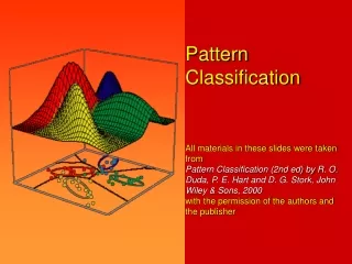
Pattern ClassificationAll materials in these slides were taken from Pattern Classification (2nd ed) by R. O. Duda, P. E. Hart and D. G. Stork, John Wiley & Sons, 2000with the permission of the authors and the publisher

Chapter 6: Multilayer Neural Networks (Sections 1-5, 8) Introduction Feedforward Operation and Classification Backpropagation Algorithm Error Surfaces Backpropagation as Feature Mapping 8. Practical Techniques for Improving Backpropagation

1. Introduction • Goal: Classify objects by learning nonlinearity • There are many problems for which linear discriminants are insufficient for minimum error • In previous methods, the central difficulty was the choice of the appropriate nonlinear functions • A “brute” approach might be to select a complete basis set such as all polynomials; such a classifier would require too many parameters to be determined from a limited number of training samples Pattern Classification, Chapter 6

There is no automatic method for determining the nonlinearities when no information is provided to the classifier • In using the multilayer Neural Networks, the form of the nonlinearity is learned from the training data Pattern Classification, Chapter 6

2. Feedforward Operation and Classification • A three-layer neural network consists of an input layer, a hidden layer and an output layer interconnected by modifiable weights represented by links between layers Pattern Classification, Chapter 6

Pattern Classification, Chapter 6

A single “bias unit” is connected to each unit other than the input units • Net activation:where the subscript i indexes units in the input layer, j in the hidden; wjidenotes the input-to-hidden layer weights at the hidden unit j. (In neurobiology, such weights or connections are called “synapses”) • Each hidden unit emits an output that is a nonlinear function of its activation, that is: yj = f(netj) Pattern Classification, Chapter 6

Figure 6.1 shows a simple threshold function • The function f(.) is also called the activation function or “nonlinearity” of a unit. There are more general activation functions with desirables properties • Each output unit similarly computes its net activation based on the hidden unit signals as: where the subscript k indexes units in the ouput layer and nHdenotes the number of hidden units Pattern Classification, Chapter 6

More than one output are referred zk. An output unit computes the nonlinear function of its net, emitting zk = f(netk) • In the case of c outputs (classes), we can view the network as computing c discriminants functions zk = gk(x) and classify the input x according to the largest discriminant function gk(x)  k = 1, …, c • The three-layer network with the weights listed in fig. 6.1 solves the XOR problem Pattern Classification, Chapter 6

The hidden unit y1 computes the boundary:  0  y1 = +1 x1 + x2 + 0.5 = 0 < 0  y1 = -1 • The hidden unit y2 computes the boundary:  0  y2 = +1 x1 + x2 -1.5 = 0 < 0  y2 = -1 • The final output unit emits z1 = +1  y1 = +1 and y2 = +1 zk = y1and not y2 = (x1 or x2) and not (x1 and x2) = x1 XOR x2 which provides the nonlinear decision of fig. 6.1 Pattern Classification, Chapter 6

General Feedforward Operation – case of c output units • Hidden units enable us to express more complicated nonlinear functions and thus extend the classification • The activation function does not have to be a sign function, it is often required to be continuous and differentiable • We can allow the activation in the output layer to be different from the activation function in the hidden layer or have different activation for each individual unit • We assume for now that all activation functions to be identical Pattern Classification, Chapter 6

Expressive Power of multi-layer Networks Question: Can every decision be implemented by a three-layer network described by equation (1) ?Answer: Yes (due to A. Kolmogorov) “Any continuous function from input to output can be implemented in a three-layer net, given sufficient number of hidden units nH, proper nonlinearities, and weights.” for properly chosen functions jand ij Pattern Classification, Chapter 6

Each of the 2n+1 hidden units jtakes as input a sum of d nonlinear functions, one for each input feature xi • Each hidden unit emits a nonlinear function jof its total input • The output unit emits the sum of the contributions of the hidden units Unfortunately: Kolmogorov’s theorem tells us very little about how to find the nonlinear functions based on data; this is the central problem in network-based pattern recognition Pattern Classification, Chapter 6

3. Backpropagation Algorithm • Any function from input to output can be implemented as a three-layer neural network • These results are of greater theoretical interest than practical, since the construction of such a network requires the nonlinear functions and the weight values which are unknown! Pattern Classification, Chapter 6

Our goal now is to set the interconnexion weights based on the training patterns and the desired outputs • In a three-layer network, it is a straightforward matter to understand how the output, and thus the error, depend on the hidden-to-output layer weights • The power of backpropagation is that it enables us to compute an effective error for each hidden unit, and thus derive a learning rule for the input-to-hidden weights, this is known as: The credit assignment problem Pattern Classification, Chapter 6

Network have two modes of operation: • Feedforward The feedforward operations consists of presenting a pattern to the input units and passing (or feeding) the signals through the network in order to get outputs units (no cycles!) • Learning The supervised learning consists of presenting an input pattern and modifying the network parameters (weights) to reduce distances between the computed output and the desired output Pattern Classification, Chapter 6

Network Learning • Let tk be the k-th target (or desired) output and zk be the k-th computed output with k = 1, …, c and w represents all the weights of the network • The training error: • The backpropagation learning rule is based on gradient descent • The weights are initialized with pseudo-random values and are changed in a direction that will reduce the error: Pattern Classification, Chapter 6

where  is the learning rate which indicates the relative size of the change in weights w(m +1) = w(m) + w(m) where m is the m-th pattern presented • Error on the hidden–to-output weights where the sensitivity of unit k is defined as: and describes how the overall error changes with the activation of the unit’s net Pattern Classification, Chapter 6

Since netk = wkt.y therefore: Conclusion: the weight update (or learning rule) for the hidden-to-output weights is: wkj = kyj = (tk – zk) f’ (netk)yj • Error on the input-to-hidden units Pattern Classification, Chapter 6

However, Similarly as in the preceding case, we define the sensitivity for a hidden unit: which means that:“The sensitivity at a hidden unit is simply the sum of the individual sensitivities at the output units weighted by the hidden-to-output weights wkj; all multipled by f’(netj)” Conclusion: The learning rule for the input-to-hidden weights is: Pattern Classification, Chapter 6

Starting with a pseudo-random weight configuration, the stochastic backpropagation algorithm can be written as: Begininitialize nH; w, criterion , , m  0 do m  m + 1 xm  randomly chosen pattern wji  wji + jxi; wkj  wkj + kyj until ||J(w)|| <  return w End Pattern Classification, Chapter 6

Stopping criterion • The algorithm terminates when the change in the criterion function J(w) is smaller than some preset value  • There are other stopping criteria that lead to better performance than this one • So far, we have considered the error on a single pattern, but we want to consider an error defined over the entirety of patterns in the training set • The total training error is the sum over the errors of n individual patterns Pattern Classification, Chapter 6

Stopping criterion (cont.) • A weight update may reduce the error on the single pattern being presented but can increase the error on the full training set • However, given a large number of such individual updates, the total error of equation (1) decreases Pattern Classification, Chapter 6

Learning Curves • Before training starts, the error on the training set is high; through the learning process, the error becomes smaller • The error per pattern depends on the amount of training data and the expressive power (such as the number of weights) in the network • The average error on an independent test set is always higher than on the training set, and it can decrease as well as increase • A validation set is used in order to decide when to stop training ; we do not want to overfit the network and decrease the power of the classifier generalization“we stop training at a minimum of the error on the validation set” Pattern Classification, Chapter 6

4. Error Surfaces • We can gain understanding and intuition about the backpropagation algorithm by studying error surfaces • The network tries to find the global minimum • But local minima can be a problem • The presence of plateaus can also be a problem Pattern Classification, Chapter 6

Consider the simplest three-layer nonlinear network with a single global minimum Pattern Classification, Chapter 6

Consider the same network with a problem that is not linearly separable Pattern Classification, Chapter 6

Consider a solution to the XOR problem Pattern Classification, Chapter 6

5. Backpropagation as Feature Mapping • Because the hidden-to-output layer leads to a linear discriminant, the novel computational power provided by multilayer neural nets can be attributed to the nonlinear warping of the input to the representation at the hidden units Pattern Classification, Chapter 6

Because the hidden-to-output weights => linear discriminant, the input-to-hidden weights are most instructive Pattern Classification, Chapter 6

8. Practical Techniques for Improving Backpropagation • Activation Function • Must be nonlinear • Must saturate – have a maximum and minimum • Must be continuous and smooth • Must be monotonic • Sigmoid class of functions provide these properties Pattern Classification, Chapter 6

2. Parameters for the Sigmoid Pattern Classification, Chapter 6

3. Scaling Input Data standardization: • The full data set should be scaled to have the same variance in each feature component Example of importance of standardization • In the fish classification chapter 1 example, suppose the fish weight is measured in grams and the fish length in meters • The weight would be orders of magnitude larger than the length Pattern Classification, Chapter 6

4. Target Values Reasonable target values are +1 and -1 For example, for a pattern in class 3, use target vector (-1, -1, +1, -1) Pattern Classification, Chapter 6

5. Training with Noise When the training set is small, additional (surrogate) training patterns can be generated by adding noise to the true training patterns. This helps most classification methods except for highly local classifiers such as kNN Pattern Classification, Chapter 6

6. Manufacturing Data As with training with noise, manufactured data can be used with a wide variety of pattern classification methods. Manufactured training data, however, usually adds more information than Gaussian noise. • For example, in OCR additional training patterns could be generated by slight rotations or line thickening of the the true training patterns Pattern Classification, Chapter 6

7. Number of Hidden Units Pattern Classification, Chapter 6

8. Initializing Weights Initial weights cannot be zero because no learning would take place In setting weights in a given layer, usually choose weights randomly from a single distribution to help ensure uniform learning • Uniform learning is when all weights reach their final equilibrium values at about the same time Pattern Classification, Chapter 6

9. Learning Rates Pattern Classification, Chapter 6

10. Momentum Pattern Classification, Chapter 6

11. Weight Decay After each weight update, every weight is simply “decayed” or shrunk wnew = wold (1 - e) Although there is no principled reason, weight decay helps in most cases Pattern Classification, Chapter 6

12. Hints For example, in OCR the hints might be straight line and curved characters. Hints are a special benefit of neural networks. Pattern Classification, Chapter 6

Chapter 6: Multilayer Neural Networks (Sections 1-5, 8)