Lecture 7 Artificial neural networks: Supervised learning
1.48k likes | 2.41k Vues
Lecture 7 Artificial neural networks: Supervised learning. Introduction, or how the brain works The neuron as a simple computing element The perceptron Multilayer neural networks Accelerated learning in multilayer neural networks The Hopfield network

Lecture 7 Artificial neural networks: Supervised learning
E N D
Presentation Transcript
Lecture 7 Artificial neural networks: Supervised learning • Introduction, or how the brain works • The neuron as a simple computing element • The perceptron • Multilayer neural networks • Accelerated learning in multilayer neural networks • The Hopfield network • Bidirectional associative memories (BAM) • Summary
Introduction, or how the brain works Machine learning involves adaptive mechanisms that enable computers to learn from experience, learn by example and learn by analogy. Learning capabilities can improve the performance of an intelligent system over time. The most popular approaches to machine learning are artificial neural networks and genetic algorithms. This lecture is dedicated to neural networks.
A neural network can be defined as a model of reasoning based on the human brain. The brain consists of a densely interconnected set of nerve cells, or basic information-processing units, called neurons. • The human brain incorporates nearly 10 billion neurons and 60 trillion connections, synapses, between them. By using multiple neurons simultaneously, the brain can perform its functions much faster than the fastest computers in existence today.
Each neuron has a very simple structure, but an army of such elements constitutes a tremendous processing power. • A neuron consists of a cell body, soma, a number of fibers called dendrites, and a single long fiber called the axon.
Our brain can be considered as a highly complex, non-linear and parallel information-processing system. • Information is stored and processed in a neural network simultaneously throughout the whole network, rather than at specific locations. In other words, in neural networks, both data and its processing are global rather than local. • Learning is a fundamental and essential characteristic of biological neural networks. The ease with which they can learn led to attempts to emulate a biological neural network in a computer.
An artificial neural network consists of a number of very simple processors, also called neurons, which are analogous to the biological neurons in the brain. • The neurons are connected by weighted links passing signals from one neuron to another. • The output signal is transmitted through the neuron’s outgoing connection. The outgoing connection splits into a number of branches that transmit the same signal. The outgoing branches terminate at the incoming connections of other neurons in the network.
I n p u t S i g n a l s O u t p u t S i g n a l s Architecture of a typical artificial neural network
The neuron as a simple computing element Diagram of aneuron
The neuron computes the weighted sum of the input signals and compares the result with a threshold value, q. If the net input is less than the threshold, the neuron output is –1. But if the net input is greater than or equal to the threshold, the neuron becomes activated and its output attains a value +1. • The neuron uses the following transfer or activation function: • This type of activation function is called a sign function.
Can a single neuron learn a task? • In 1958, Frank Rosenblatt introduced a training algorithm that provided the first procedure for training a simple ANN: a perceptron. • The perceptron is the simplest form of a neural network. It consists of a single neuron with adjustable synaptic weights and a hard limiter.
ThePerceptron • The operation of Rosenblatt’s perceptron is based on the McCulloch and Pitts neuron model. The model consists of a linear combiner followed by a hard limiter. • The weighted sum of the inputs is applied to the hard limiter, which produces an output equal to +1 if its input is positive and -1 if it is negative.
The aim of the perceptron is to classify inputs, x1, x2, . . ., xn, into one of two classes, say A1 and A2. • In the case of an elementary perceptron, the n-dimensional space is divided by a hyperplane into two decision regions. The hyperplane is defined by the linearly separable function:
How does the perceptron learn its classification tasks? This is done by making small adjustments in the weights to reduce the difference between the actual and desired outputs of the perceptron. The initial weights are randomly assigned, usually in the range [-0.5, 0.5], and then updated to obtain the output consistent with the training examples.
If at iteration p, the actual output is Y(p) and the desired output is Yd(p), then the error is given by: where p = 1, 2, 3, . . . • Iteration p here refers to the pth training example presented to the perceptron. • If the error, e(p), is positive, we need to increase perceptron output Y(p), but if it is negative, we need to decrease Y(p).
. . a The perceptron learning rule where p = 1, 2, 3, . . . a is the learning rate, a positive constant less than unity. The perceptron learning rule was first proposed by Rosenblatt in 1960. Using this rule we can derive the perceptron training algorithm for classification tasks.
Perceptron’s training algorithm Step 1: Initialisation Set initial weights w1, w2,…, wnand threshold q to random numbers in the range [-0.5, 0.5]. If the error, e(p), is positive, we need to increase perceptronoutput Y(p), but if it is negative, we need to decrease Y(p).
Perceptron’s training algorithm (continued) Step 2: Activation Activate the perceptron by applying inputs x1(p), x2(p),…, xn(p) and desired output Yd(p). Calculate the actual output at iteration p = 1 where n is the number of the perceptron inputs, and step is a step activation function.
. Perceptron’s training algorithm (continued) Step 3: Weight training Update the weights of the perceptron where Dwi(p) is the weight correction at iteration p. The weight correction is computed by the delta rule: Step 4: Iteration Increase iteration p by one, go back to Step 2 and repeat the process until convergence.
(a) AND (x1Ç x2) Two-dimensional plots of basic logical operations A perceptron can learn the operations AND and OR, but not Exclusive-OR.
Multilayerneuralnetworks • A multilayer perceptron is a feedforward neural network with one or more hidden layers. • The network consists of an input layer of source neurons, at least one middle or hidden layer of computational neurons, and an output layer of computational neurons. • The input signals are propagated in a forward direction on a layer-by-layer basis.
I n p u t S i g n a l s O u tp u t S i g n a l s Multilayer perceptron with two hidden layers
What does the middle layer hide? • A hidden layer “hides” its desired output. Neurons in the hidden layer cannot be observed through the input/output behaviour of the network. There is no obvious way to know what the desired output of the hidden layer should be. • Commercial ANNs incorporate three and sometimes four layers, including one or two hidden layers. Each layer can contain from 10 to 1000 neurons. Experimental neural networks may have five or even six layers, including three or four hidden layers, and utilise millions of neurons.
Back-propagation neural network • Learning in a multilayer network proceeds the same way as for a perceptron. • A training set of input patterns is presented to the network. • The network computes its output pattern, and if there is an error - or in other words a difference between actual and desired output patterns - the weights are adjusted to reduce this error.
In a back-propagation neural network, the learning algorithm has two phases. • First, a training input pattern is presented to the network input layer. The network propagates the input pattern from layer to layer until the output pattern is generated by the output layer. • If this pattern is different from the desired output, an error is calculated and then propagated backwards through the network from the output layer to the input layer. The weights are modified as the error is propagated.
The back-propagation training algorithm Step 1: Initialisation Set all the weights and threshold levels of the network to random numbers uniformly distributed inside a small range: where Fiis the total number of inputs of neuron i in the network. The weight initialisation is done on a neuron-by-neuron basis.
Step 2: Activation Activate the back-propagation neural network by applying inputs x1(p), x2(p),…, xn(p) and desired outputs yd,1(p), yd,2(p),…, yd,n(p). (a) Calculate the actual outputs of the neurons in the hidden layer: where n is the number of inputs of neuron j in the hidden layer, and sigmoid is the sigmoid activation function.
Step 2: Activation (continued) (b) Calculate the actual outputs of the neurons in the output layer: where m is the number of inputs of neuron k in the output layer.
Step 3: Weight training Update the weights in the back-propagation network propagating backward the errors associated with output neurons. (a) Calculate the error gradient for the neurons in the output layer: where Calculate the weight corrections: Update the weights at the output neurons:
Step 3: Weight training (continued) (b) Calculate the error gradient for the neurons in the hidden layer: Calculate the weight corrections: Update the weights at the hidden neurons:
Step 4: Iteration Increase iteration p by one, go back to Step 2 and repeat the process until the selected error criterion is satisfied. As an example, we may consider the three-layer back-propagation network. Suppose that the network is required to perform logical operation Exclusive-OR. Recall that a single-layer perceptron could not do this operation. Now we will apply the three-layer net.
The effect of the threshold applied to a neuron in the hidden or output layer is represented by its weight, q, connected to a fixed input equal to -1. • The initial weights and threshold levels are set randomly as follows: w13= 0.5, w14= 0.9, w23= 0.4, w24 = 1.0, w35 = -1.2, w45 = 1.1, q3 = 0.8, q4 = -0.1 and q5 = 0.3.
We consider a training set where inputs x1 and x2 are equal to 1 and desired output yd,5 is 0. The actual outputs of neurons 3 and 4 in the hidden layer are calculated as • Now the actual output of neuron 5 in the output layer is determined as: • Thus, the following error is obtained:
The next step is weight training. To update the weights and threshold levels in our network, we propagate the error, e, from the output layer backward to the input layer. • First, we calculate the error gradient for neuron 5 in the output layer: • Then we determine the weight corrections assuming that the learning rate parameter, a, is equal to 0.1:
Next we calculate the error gradients for neurons 3 and 4 in the hidden layer: • We then determine the weight corrections:
At last, we update all weights and threshold: • The training process is repeated until the sum ofsquared errors is less than 0.001.
Sum-Squared Error Learning curve for operation Exclusive-OR
Network represented by McCulloch-Pitts model for solving the Exclusive-OR operation
Decision boundaries • Decisionboundary constructed by hidden neuron 3; (b) Decision boundary constructed by hidden neuron 4; (c) Decision boundaries constructed by the complete three-layer network
Accelerated learning in multilayer neural networks • A multilayer network learns much faster when the sigmoidal activation function is represented by a hyperbolic tangent: where a and bare constants. Suitable values for a and b are: a = 1.716 and b = 0.667
We also can accelerate training by including a momentum term in the delta rule: where b is a positive number (0 £ b < 1) called the momentum constant. Typically, the momentum constant is set to 0.95. This equation is called the generalised delta rule.
Learning Rate Learning with momentum for operation Exclusive-OR