Download

1 / 99
1.03k likes | 1.26k Vues
Hierarchical Neural Networks for Object Recognition and Scene “Understanding” . From Mick Thomure , Ph.D. Defense, PSU, 2013 . Object Recognition. Task : Given an image containing foreground objects, predict one of a set of known categories. “Motorcycle”. “Fox”. “Airplane”.

E N D
Hierarchical Neural Networks for Object Recognition and Scene “Understanding”
From Mick Thomure, Ph.D. Defense,PSU, 2013 Object Recognition Task: Given an image containing foreground objects, predict one of a set of known categories. “Motorcycle” “Fox” “Airplane”
From Mick Thomure, Ph.D. Defense,PSU, 2013 Selectivity: ability to distinguish categories “No-Bird” “Bird”
From Mick Thomure, Ph.D. Defense,PSU, 2013 Invariance: tolerance to variation In-category Variation Rotation Translation Scaling
From: http://play.psych.mun.ca/~jd/4051/The%20Primary%20Visual%20Cortex.ppt
From: http://psychology.uwo.ca/fmri4newbies/Images/visualareas.jpg
Hubel and Wiesel’s discoveries • Based on single-cell recordings in cats and monkeys • Found that in V1, most neurons are one of the following types: • Simple: Respond to edges at particular locations and orientations within the visual field • Complex: Also respond to edges, but are more tolerant of location and orientation variation than simple cells • Hypercomplex or end-stopped: Are selective for a certain length of contour Adapted from: http://play.psych.mun.ca/~jd/4051/The%20Primary%20Visual%20Cortex.ppt
Neocognitron • Hierarchical neural network proposed by K. Fukushima in 1980s. • Inspired by Hubel and Wiesel’s studies of visual cortex.
HMAX Riesenhuber, M. & Poggio, T. (1999),“Hierarchical Models of Object Recognition in Cortex”Serre, T., Wolf, L., Bileschi, S., Risenhuber, M., and Poggio, T. (2006),“Robust Object Recognition with Cortex-Like Mechanisms” • HMAX: A hierarchical neural-network model of object recognition. • Meant to model human vision at level of “immediate recognition” capabilities of ventral visual pathway, independent of attention or other top-down processes. • Inspired by earlier “Neocognitron” model of Fukushima (1980)
General ideas behind model • “Immediate” visual processing is feedforward and hierachical: low levels detect simple features, which are combined hierarchically into increasingly complex features to be detected • Layers of hierarchy alternate between “sensitivity” (to detecting features) and “invariance” (to position, scale, orientation) • Size of receptive fields increases along the hierarchy • Degree of invariance increases along the hierarchy
From Mick Thomure, Ph.D. Defense,PSU, 2013 HMAX State-of-the-art performance on common benchmarks. 1500+ references to HMAX since 1999. Many extensions and applications • Biometrics • Remote sensing • Modeling visual processing in biology Processing
From Mick Thomure, Ph.D. Defense,PSU, 2013 Template Matching: selectivity for visual patterns Pooling: invariance to transformation by combining multiple inputs Pooling Template Template Matching ON Input Pooling Template Template Matching OFF
From Mick Thomure, Ph.D. Defense,PSU, 2013 S1 Layer: edge detection Edge Detectors S1 Input
From Mick Thomure, Ph.D. Defense,PSU, 2013 C1 Layer: local pooling Some tolerance to position and scale. C1 S1 Input
From Mick Thomure, Ph.D. Defense,PSU, 2013 S2 Layer: prototype matching Match learned dictionary of shape prototypes S2 C1 S1 Input
From Mick Thomure, Ph.D. Defense,PSU, 2013 C2 Layer: global pooling Activity is max response to S2 prototype at any location or scale. C2 S2 C1 S1 Input
From Mick Thomure, Ph.D. Defense,PSU, 2013 Properties of C2 Activity Prototype • Activity reflects degree of match • Location and size do not matter • Only best match counts Activation Input Input Input
From Mick Thomure, Ph.D. Defense,PSU, 2013 Properties of C2 Activity Prototype • Activity reflects degree of match • Location and size do not matter • Only best match counts Activation Input Input
From Mick Thomure, Ph.D. Defense,PSU, 2013 Properties of C2 Activity Prototype • Activity reflects degree of match • Location and size do not matter • Only best match counts Activation Input Input Input
From Mick Thomure, Ph.D. Defense,PSU, 2013 Classifier: predict object category Output of C2 layer forms a feature vector to be classified. Some possible classifiers: SVM Boosted Decision Stumps Logistic Regression C2 S2 C1 S1 Input
Gabor Filters Gabor filter: Essentially a localized Fourier transform, focusing on a particular spatial frequency, orientation, and scale in the image. Filter has associated frequency , scale s, and orientation . Response measures extent to which is present at orientation at scale s centered about pixel (x,y).
Theta = 0 Lambda = 5 Theta = 0 Lambda = 10 Theta = 0 Lambda = 15 Theta = 0 Lambda = 10 Theta = 45 Lambda = 10 Theta = 90 Lambda = 10 http://matlabserver.cs.rug.nl/cgi-bin/matweb.exe
Examples of Gabor filters of different orientations and scales From http://www.cs.cmu.edu/~efros/courses/LBMV07/presentations/0130SerreC2Features.ppt
HMAX: How to set parameters for Gabor filters • Sample parameter space • Apply corresponding filters to stimuli commonly used to probe cortical cells (i.e., gratings, bars, edges) • Select parameter values that capture the tuning properties of V1 simple cells, as reported in the neuroscience literature
Learning V1 Simple Cells via Sparse CodingOlshausen & Field, 1996 • Hypotheses: • Any natural image I(x,y) can be represented by a linear superposition of (not necessarily orthogonal) basis functions, ϕ(x,y): • The ϕispan the image space(i.e., any image can be reconstructed with appropriate choice of ai) • The aiare as statistically independent as possible • Any natural image has a representation that is sparse (i.e., can be represented by a small number of non-zero ai)
Test of hypothesis: Use these criteria to learn a set of ϕifrom a database of natural images. • Use gradient descent, with the following cost function: cost of non-sparseness (using too many ai), where S is a nonlinear function and σiis a scaling constant cost of incorrect reconstruction
Training set: a set of 12x12 image patches from natural images. • Start with large random set (144) of ϕi • For each patch, • Find set of ai to minimize E with respect to ai • With these ai, Update ϕiusing this learning rule: where
From http://redwood.berkeley.edu/bruno/papers/current-opinion.pdf These resemble receptive fields of V1 simple cells: they are (1) localized, (2) orientation-specific, (3) frequency and scale-specific
S1 units: Gabor filters (one per pixel) 16 scales / frequencies, 4 orientations (0, 45, 90, 135). Units form a pyramid of scales, from 7x7 to 37x37 pixels in steps of two pixels. Response of an S1 unit is absolute value of filter response.
C1 unit: Maximum value of group of S1 units, pooled over slightly different positions and scales 8 scales / frequencies, 4 orientations
The S1 and C1 model parameters are meant to match empirical neuroscience data. From S. Bileschi, Ph.D. Thesis
S2 layer • Recall that each S1 unit responds to an oriented edge at a particular scale • Each S2 unit responds to a particular group of oriented edges at various scales, i.e., a shape • S1 units were chosen to cover a “full” range of scales and orientations • How can we choose S2 units to cover a “full” range of shapes?
HMAX’s answer: Choose S2 shapes by randomly sampling patches from “training images”
HMAX’s answer: Choose S2 shapes by randomly sampling patches from “training images” Extract C1 features in each selected patch. This gives a p×p×4 array, for 4 orientations.
S2 prototype Pi , with 4 orientations Scale 1 Scale 2 Scale 3 Scale 4 Scale 8 Scale 5 Scale 6 Scale 7
S2 prototype Pi , with 4 orientations Calculate similarity between Pi and patches in input image, independently at each position and each scale. Input image to classify: C1 layer: 4 orientations, 8 scales Scale 1 Scale 2 Scale 3 Scale 4 Scale 8 Scale 5 Scale 6 Scale 7
Similarity (radial basis function): S2 prototype Pi , with 4 orientations Calculate similarity between Pi and patches in input image, independently at each position and each scale. Input image to classify: C1 layer: 4 orientations, 8 scales Scale 1 Scale 4 Scale 2 Scale 3 Scale 8 Scale 5 Scale 6 Scale 7
Similarity (radial basis function): S2 prototype Pi , with 4 orientations Calculate similarity between Pi and patches in input image, independently at each position and each scale. Input image to classify: C1 layer: 4 orientations, 8 scales Scale 1 Scale 4 Scale 2 Scale 3 Scale 8 Scale 5 Scale 6 Scale 7 Result: At each position in C1 layer of input image, we have an array of 4x8 values. Each value represents the “degree” to which shape Piis present at the given position at the given orientation and scale.
Similarity (radial basis function): S2 prototype Pi , with 4 orientations Calculate similarity between Pi and patches in input image, independently at each position and each scale. Input image to classify: C1 layer: 4 orientations, 8 scales Scale 1 Scale 4 Scale 2 Scale 3 Scale 8 Scale 5 Scale 6 Scale 7 Result: At each position in C1 layer of input image, we have an array of 4x8 values. Each value represents the “degree” to which shape Piis present at the given position at the given scale. Now, repeat this process for each Pi, to get N such arrays.
C2 unit: For each Pi, calculate maximum value over all positions, orientations, and scales. Result is N values, corresponding to the N prototypes.
Feature vector representing image SVM classification: To classify input image (e.g., “face” or “not face”), give C2 values to a trained support vector machine (SVM). Support Vector Machine classification
Boosting classification: To classify input image (e.g., “face” or “not face”), give C2 values to a trained classifier trained by Adaboost. Feature vector representing image Adaboost Classifier classification
Visual tasks: (1) Part-based object detection: Detect different types of “part-based” objects, either alone or in “clutter”. Data sets contain images that either contain or do not contain a single instance of the target object. Task is to decide whether the target object is present or absent. (2) Texture-based object recognition: Recognize different types of “texture-based” objects (e.g., grass, trees, buildings, roads). Task is to classify each pixel with an object label. (3) Whole-Scene Recognition: Recognize all objects (“part-based” and “texture-based”) in a scene.
Databases • Caltech 5 (Five object categories: leaves, cars, faces, airplanes, motocycles) • Caltech 101 (101 object categories) • MIT Streetscenes • MIT car and face databases
Sample images from the MIT Streetscenes database