6.870 Object Recognition and Scene Understanding

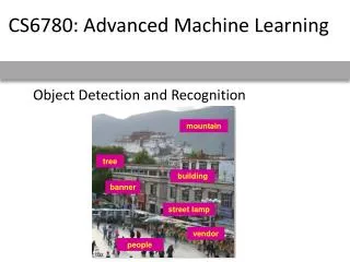
1. http://people.csail.mit.edu/torralba/courses/6.870/6.870.recognition.htmhttp://people.csail.mit.edu/torralba/courses/6.870/6.870.recognition.htm 6.870 Object Recognition and Scene Understanding Lecture 2 Overview on object recognition and one practical example

2. Wednesday • Nicolas Pinto: Template matching and gradient histograms • Jenny Yuen: Demo of Dalal&Triggs detector and interface with LabelMe

3. Find the chair in this image This is a chair Object recognitionIs it really so hard? Output of normalized correlation

4. Find the chair in this image Object recognitionIs it really so hard? Pretty much garbage Simple template matching is not going to make it My biggest concern while making this slide was: how do I justify 50 years of research, and this course, if this experiment did work?

5. Find the chair in this image Object recognitionIs it really so hard? A “popular method is that of template matching, by point to point correlation of a model pattern with the image pattern. These techniques are inadequate for three-dimensional scene analysis for many reasons, such as occlusion, changes in viewing angle, and articulation of parts.” Nivatia & Binford, 1977.

6. So, let’s make the problem simpler:Block world Nice framework to develop fancy math, but too far from reality… Object Recognition in the Geometric Era: a Retrospective. Joseph L. Mundy. 2006

7. Binford and generalized cylinders Object Recognition in the Geometric Era: a Retrospective. Joseph L. Mundy. 2006

8. Binford and generalized cylinders

9. Recognition by components Irving Biederman Recognition-by-Components: A Theory of Human Image Understanding. Psychological Review, 1987.

10. Recognition by components The fundamental assumption of the proposed theory, recognition-by-components (RBC), is that a modest set of generalized-cone components, called geons(N = 36), can be derived from contrasts of five readily detectable properties of edges in a two-dimensional image: curvature, collinearity, symmetry, parallelism, and cotermination. The “contribution lies in its proposal for a particular vocabulary of components derived from perceptual mechanisms and its account of how an arrangement of these components can access a representation of an object in memory.”

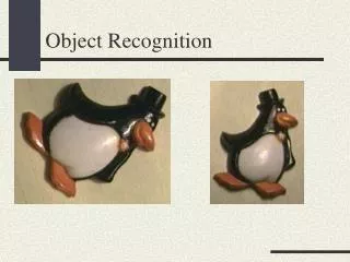
11. A do-it-yourself example • We know that this object is nothing we know • We can split this objects into parts that everybody will agree • We can see how it resembles something familiar: “a hot dog cart” • “The naive realism that emerges in descriptions of nonsense objects may be reflecting the workings of a representational system by which objects are identified.”

12. Hypothesis • Hypothesis: there is a small number of geometric components that constitute the primitive elements of the object recognition system (like letters to form words). • “The particular properties of edges that are postulated to be relevant to the generation of the volumetric primitives have the desirable properties that they are invariant over changes in orientation and can be determined from just a few points on each edge.” • Limitation: “The modeling has been limited to concrete entities with specified boundaries.” (count nouns) – this limitation is shared by many modern object detection algorithms.

13. Constraints on possible models of recognition • Access to the mental representation of an object should not be dependent on absolute judgments of quantitative detail • The information that is the basis of recognition should be relatively invariant with respect to orientation and modest degradation. • Partial matches should be computable. A theory of object interpretation should have some principled means for computing a match for occluded, partial, or new exemplars of a given category.

14. Stages of processing “Parsing is performed, primarily at concave regions, simultaneously with a detection of nonaccidental properties.”

15. image ? e.g., Freeman, “the generic viewpoint assumption”, 1994 Non accidental properties Certain properties of edges in a two-dimensional image are taken by the visual system as strong evidence that the edges in the three-dimensional world contain those same properties. Non accidental properties, (Witkin & Tenenbaum,1983): Rarely be produced by accidental alignments of viewpoint and object features and consequently are generally unaffected by slight variations in viewpoint.

16. Examples: • Colinearity • Smoothness • Symmetry • Parallelism • Cotermination

17. The high speed and accuracy of determining a given nonaccidental relation {e.g., whether some pattern is symmetrical) should be contrasted with performance in making absolute quantitative judgments of variations in a single physical attribute, such as length of a segment or degree of tilt or curvature. Object recognition is performed by humans in around 100ms.

18. Recoverable Unrecoverable “If contours are deleted at a vertex they can be restored, as long as there is no accidental filling-in. The greater disruption from vertex deletion is expected on the basis of their importance as diagnostic image features for the components.”

19. From generalized cylinders to GEONS “From variation over only two or three levels in the nonaccidental relations of four attributes of generalized cylinders, a set of 36 GEONS can be generated.” Geons represent a restricted form of generalized cylinders.

20. More GEONS

21. Objects and their geons

22. Scenes and geons Mezzanotte & Biederman

23. The importance of spatial arrangement

24. Supercuadrics Introduced in computer vision by A. Pentland, 1986.

25. What is missing? The notion of geometric structure. Although they were aware of it, the previous works put more emphasis on defining the primitive elements than modeling their geometric relationships.

26. Parts and Structure approaches • With a different perspective, these models focused more on the geometry than on defining the constituent elements: • Fischler & Elschlager 1973 • Yuille ‘91 • Brunelli & Poggio ‘93 • Lades, v.d. Malsburg et al. ‘93 • Cootes, Lanitis, Taylor et al. ‘95 • Amit & Geman ‘95, ‘99 • Perona et al. ‘95, ‘96, ’98, ’00, ’03, ‘04, ‘05 • Felzenszwalb & Huttenlocher ’00, ’04 • Crandall & Huttenlocher ’05, ’06 • Leibe & Schiele ’03, ’04 • Many papers since 2000 Figure from [Fischler & Elschlager 73]

27. Representation • Object as set of parts • Generative representation • Model: • Relative locations between parts • Appearance of part • Issues: • How to model location • How to represent appearance • Sparse or dense (pixels or regions) • How to handle occlusion/clutter We will discuss these models more in depth next week

28. But, despite promising initial results…things did not work out so well (lack of data, processing power, lack of reliable methods for low-level and mid-level vision) Instead, a different way of thinking about object detection started making some progress: learning based approaches and classifiers, which ignored low and mid-level vision. Maybe the time is here to come back to some of the earlier models, more grounded in intuitions about visual perception.

29. A simple object detector • Simple but contains some of same basic elements of many state of the art detectors. • Based on boosting which makes all the stages of the training and testing easy to understand. Most of the slides are from the ICCV 05 short course http://people.csail.mit.edu/torralba/shortCourseRLOC/

30. (The artist) 0.1 0.05 0 0 10 20 30 40 50 60 70 • Discriminative model (The lousy painter) 1 0.5 0 0 10 20 30 40 50 60 70 x = data • Classification function 1 -1 0 10 20 30 40 50 60 70 80 x = data Discriminative vs. generative • Generative model x = data

31. Background Computer screen Bag of image patches In some feature space Discriminative methods Object detection and recognition is formulated as a classification problem. The image is partitioned into a set of overlapping windows … and a decision is taken at each window about if it contains a target object or not. Decision boundary Where are the screens?

32. Discriminative methods Neural networks Nearest neighbor 106 examples LeCun, Bottou, Bengio, Haffner 1998 Rowley, Baluja, Kanade 1998 … Shakhnarovich, Viola, Darrell 2003 Berg, Berg, Malik 2005 … Conditional Random Fields Support Vector Machines and Kernels Guyon, Vapnik Heisele, Serre, Poggio, 2001 … McCallum, Freitag, Pereira 2000 Kumar, Hebert 2003 …

33. Classification function Where belongs to some family of functions Formulation • Formulation: binary classification … x1 x2 x3 … xN xN+1 xN+2 xN+M … Features x = -1 +1 -1 -1 ? ? ? y = Labels Training data: each image patch is labeled as containing the object or background Test data • Minimize misclassification error • (Not that simple: we need some guarantees that there will be generalization)

34. Overview of section • Object detection with classifiers • Boosting • Gentle boosting • Weak detectors • Object model • Object detection

35. A simple object detector with Boosting • Download • Toolbox for manipulating dataset • Code and dataset • Matlab code • Gentle boosting • Object detector using a part based model • Dataset with cars and computer monitors http://people.csail.mit.edu/torralba/iccv2005/

36. Why boosting? • A simple algorithm for learning robust classifiers • Freund & Shapire, 1995 • Friedman, Hastie, Tibshhirani, 1998 • Provides efficient algorithm for sparse visual feature selection • Tieu & Viola, 2000 • Viola & Jones, 2003 • Easy to implement, not requires external optimization tools.

37. Boosting • Defines a classifier using an additive model: Strong classifier Weak classifier Weight Features vector

38. Boosting • Defines a classifier using an additive model: • We need to define a family of weak classifiers Strong classifier Weak classifier Weight Features vector from a family of weak classifiers

39. +1 ( ) yt = -1 ( ) Boosting • It is a sequential procedure: xt=1 Each data point has a class label: xt xt=2 and a weight: wt =1

40. +1 ( ) yt = -1 ( ) Toy example Weak learners from the family of lines Each data point has a class label: and a weight: wt =1 h => p(error) = 0.5 it is at chance

41. +1 ( ) yt = -1 ( ) Toy example Each data point has a class label: and a weight: wt =1 This one seems to be the best This is a ‘weak classifier’: It performs slightly better than chance.

42. +1 ( ) yt = -1 ( ) Toy example Each data point has a class label: We update the weights: wt wt exp{-yt Ht} We set a new problem for which the previous weak classifier performs at chance again

43. +1 ( ) yt = -1 ( ) Toy example Each data point has a class label: We update the weights: wt wt exp{-yt Ht} We set a new problem for which the previous weak classifier performs at chance again

44. +1 ( ) yt = -1 ( ) Toy example Each data point has a class label: We update the weights: wt wt exp{-yt Ht} We set a new problem for which the previous weak classifier performs at chance again

45. +1 ( ) yt = -1 ( ) Toy example Each data point has a class label: We update the weights: wt wt exp{-yt Ht} We set a new problem for which the previous weak classifier performs at chance again

46. Toy example f1 f2 f4 f3 The strong (non- linear) classifier is built as the combination of all the weak (linear) classifiers.

47. Boosting • Different cost functions and minimization algorithms result is various flavors of Boosting • In this demo, I will use gentleBoosting: it is simple to implement and numerically stable.

48. Overview of section • Object detection with classifiers • Boosting • Gentle boosting • Weak detectors • Object model • Object detection

49. Boosting Boosting fits the additive model by minimizing the exponential loss Training samples The exponential loss is a differentiable upper bound to the misclassification error.

50. Exponential loss Squared error Loss 4 Misclassification error 3.5 Squared error 3 Exponential loss 2.5 2 Exponential loss 1.5 1 0.5 0 -1.5 -1 -0.5 0 0.5 1 1.5 2 yF(x) = margin