Artificial Neural Networks

1. Artificial Neural Networks Modeling Nature’s Solution

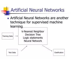
2. Want machines to learn Want to model approach after those found in nature Best learner in nature? Brain Neural Networks

3. How Do Brain’s Learn? • Vast networks of cells called neurons • Human ~100 billion neurons • Each neuron estimated to have ~1,000 connections to other neurons • Known as synaptic connections • ~100 trillion synapses Neural Networks

4. Pathways for Electrical Signals • A neuron receives input from the axons of other neurons • Dendrites form a web of possible input locations • When the incoming potentials reach a critical level the neuron fires exciting neurons downstream Neural Networks

5. Donald Hebb 1949 Psychologist: proposed that classical conditioning (Pavlovian) is possible because of individual neuron properties Proposed a mechanism for learning in biological neurons Neural Networks

6. Hebb’s Rule Let us assume that the persistence or repetition of a reverberatory activity (or "trace") tends to induce lasting cellular changes that add to its stability.… When an axon of cell A is near enough to excite a cell B and repeatedly or persistently takes part in firing it, some growth process or metabolic change takes place in one or both cells such that A's efficiency, as one of the cells firing B, is increased. Neural Networks

7. Some synaptic connections fire more easily over time Less resistance Form synaptic pathways Some form “callouses” and are more resistant to firing Repetitive Reinforcement Neural Networks

8. In a very real sense, learning can be boiled down to the process of determining the appropriate resistances between the vast network of axon to dendrite connections in the brain Learning Neural Networks

9. 1940’s Warren McCulloch and Walter Pitts Showed that networks of artificial neurons could, in principle, compute any arithmetic or logical function Warren McCulloch Walter Pitts Neural Networks

10. Abstraction • Neuron: like an electrical circuit with multiple inputs and a single output (though it can branch out to multiple locations) Σ And some threshold Dendrites Axon Neural Networks

11. Learning • Learning becomes a matter of discovering the appropriate resistance values Σ And some threshold Dendrites Axon Neural Networks

12. Computationally • Resistors become weights • Linear combination Bias W0 W1 W2 W3 Σ inputs f . . . Transfer Function Wn Neural Networks

13. 1950’s Interest sored BernardWidrow and Ted Hoff introduced a new learning rule Widrow-Hoff (still in use today) Used in the simple Perceptron neural network Neural Networks

14. 1960 Frank Rosenblatt Cornell University Created the Perceptron Computer Perceptronswere simulated on an IBM 704 First computer that could learn new skills by trial and error IEEE’s Frank Rosenblatt Award, for "outstanding contributions to the advancement of the design, practice, techniques or theory in biologically and linguistically motivated computational paradigms including but not limited to neural networks, connectionist systems, evolutionary computation, fuzzy systems, and hybrid intelligent systems in which these paradigms are contained." Neural Networks

15. Perceptron • As usual, each training instance used to adjust weights Bias W0 W1 Class Training Data W2 W3 Σ inputs f . . . Transfer Function Wn Neural Networks

16. Learning rule • Look familiar? • t is target (class) • o is output (output of perceptron) Neural Networks

17. Could do one at a time • Known as stochastic approximation to gradient descent • Known as the perceptron rule Neural Networks

18. Transfer Function • Output (remember: target – output) • Example: binary class—0 or 1 • hardlim(n) • If n < 0 return 0 • Otherwise return 1 Bias W0 W1 W2 W3 Σ inputs f . . . Transfer Function Wn Neural Networks

19. Example • Decision boundary • Red • Class 0 • Green • Class 1 W = [0.195, -0.065, 0.0186] Neural Networks

20. Classification • Decision boundary • Linear combination • Hardlim(n) • If n < 0 return 0 • Otherwise return 1 For plotting purposes Neural Networks

21. Algorithm Gradient-Descent(training_examples,η) Each training example is a pair of the form where is the vector of input values, and is the target output value, η is the learning rate (e.g. .05) • Initialize each to some small random value • Until the termination condition is met, DO • Initialize each to zero • For each in training_examples, DO • Input the instance to the unit and compute the output o • For each linear unit weight , DO • For each linear unit weight , DO Neural Networks

22. Implementation in R • Initialize each 𝑤_𝑖 to some small random value • Until the termination condition is met, DO • Initialize each ∆𝑤_𝑖 to zero • For each ⟨𝑥 ⃗,𝑡⟩ in training_examples, DO • Input the instance 𝑥 ⃗ to the unit and compute the output o • For each linear unit weight 𝑤_𝑖, DO • ∆𝑤_𝑖←𝜂(𝑡−𝑜) 𝑥_𝑖 • For each linear unit weight 𝑤_𝑖, DO • 𝑤_𝑖←𝑤_𝑖+∆𝑤_𝑖 eta = .001 deltaW = rep(0,numDims + 1) errorCount= 1 epoch = 0 while(errorCount>0){ errorCount= 0 for (idx in c(1:dim(trData)[1])){#for each trinst deltaW= 0*deltaW#init delta w to zero input = c(1,trData[idx,1:2]) #input is xy of tr output = hardlim(sum(w*input)) #run thru perceptron target = trData[idx,3] if(output != target){ errorCount=errorCount+ 1 } #calc delta w deltaW = eta*(target - output)*input w = w + deltaW } if(epoch %% 100 == 0){ abline(c(-w[1]/w[3],-w[2]/w[3]),col="yellow") } } Neural Networks

23. When did it stop? • Stopping condition? How well will it classify future instances? Neural Networks

24. What if not linearly separable • Use hardlim to train (t-o), not residual • Not minimizing square differences Neural Networks

25. Book “Perceptrons” published in 1969 (Marvin Minsky and Seymour Papert) Publicized inherent limitations of ANN’s Couldn’t solve a simple XOR problem Serious Limitations Marvin Minsky Seymour Papert Neural Networks

26. Many were influenced by Minsky and Papert Mass exodus from the field For a decade, research in ANNs lay mostly dormant Artificial Neural Networks Dead? Neural Networks

27. Far From Antagonistic Minsky and Papertdeveloped the “Society of the Mind” theory Intelligence could be a product of the interaction of non-intelligent parts Quote from Arthur C. Clarke, 2001: A Space Odyssey “Minskyand Good had shown how neural networks could be generated automatically—self replicated… Artificial brains could be grown by a process strikingly analogous to the development of a human brain. “ Neural Networks

28. The AI winter In fact, the effect was field wide More likely a combination of hype generated unreasonable expectations and several high profile AI failures Speech recognition Automatic translators Expert systems Neural Networks

29. Funding was down But, during this time… ANNs shown to be usable as memory (Kohonen networks) Stephen Grossberg developed self-organizing networks (SOMs) Not completely dead Neural Networks

30. 1980s More accessible computing Revitalization Renaissance Neural Networks

31. Two New Concepts Largely responsible for rebirth Recurrent networks; useful as associative memory Back propagation: David Rumelhart and James McClelland Answered Minsky and Papert’s criticisms Neural Networks

32. Multilayer Networks Input Units Hidden layer Output Units x1 x2 . . . xm w w w w w w w w w w w w w w w w w w Σ Σ Σ Σ Σ Σ Σ Σ Σ f f f f f f f f f . . . . . . . . . . . . . . . . . . . . . . . . . . . w w w w w w w w w Neural Networks

33. Called… Multilayer Feedforward Network Data x1 x2 . . . xm w w w w w w w w w w w w w w w w w w Σ Σ Σ Σ Σ Σ Σ Σ Σ f f f f f f f f f w w . . . . . . . . . w w w w w w w Neural Networks

34. Adjusting Weights… Must be done in the context of the current layer’s input and output But what is the “target” value for a given layer? w Base these weight adjustments on these output values w Σ f . . . w Neural Networks

35. Instead of… Working with target values, can work with error values of the node ahead • Output branches to several downstream nodes (albeit a particular input of that node) • If we start at the output end, we know how far off the mark it is (its error) w w Σ f . . . w Neural Networks

36. Non-output nodes Look at the “errors“ of the units ahead instead of target values Error based on the summation of the errors of the units to which it is tied w w Error based on target and output (t-o) w f w f Σ Σ . . . . . . w w Neural Networks

37. Backpropagation of Error Backpropagation Learning Algorithm Data x1 x2 . . . xm w w w w w w w w w w w w w w w w w w Σ Σ Σ Σ Σ Σ Σ Σ Σ f f f f f f f f f . . . . . . . . . . . . . . . . . . . . . . . . . . . w w w w w w w w w Error Neural Networks

38. Output, the calculated Y given Xi and the current values in the weight vector Error Calculations • Original gradient descent • Partial differentiation of the overall error between a predicted line and target values • Residuals—regression Target, the Y of the training data Neural Networks

39. But… • The perceptron rule switched to a stochastic approximation • And it was no longer, strictly speaking, based upon gradient descent • Hardlim non-differentiable Bias W0 W1 W2 W3 Σ inputs f . . . Transfer Function Wn Neural Networks

40. In order… • …to return to a mathematically rigorous solution • Switched transfer functions • Sigmoid • Can determine instantaneous slopes Binary (Logistic) Sigmoid Function fbs(nk) 1 nk 0 -5 5 Neural Networks

41. Delta weights • Derivation Where is the error on training example d, summed over all output units in the network Outputs is the set of output units in the network, is the target value of the unit k for training example d, and is the output of unit k given training example d Neural Networks

42. Stochastic gradient descent rule • Some terms the ith input to unit j the weight associated with the ith input to unit j (the weighted sum of inputs for unit j) the output computed by unit j the target output for unit j the sigmoid function the set of units in the final layer of the network the set of units whose immediate inputs include the output of unit j Neural Networks

43. Derivation Chain rule (weight can influence the rest of the network only through ) can influence the network only through First term Neural Networks

44. Derivation The derivatives of will be zero for all output units k except when k = j. They therefore drop the summation and set k=j Second term. Since the derivative of is just the derivative of the sigmoid function, which they have already noted is equal to With some substitutions Neural Networks

45. For output units • Looks a little different • There are some “1-’s”and extra “o’s” • But… Neural Networks

46. Hidden Units • We are interested in the error associated with a hidden unit Error associated with a unit: Will designate as (the negative sign useful for direction of change computations) Neural Networks

47. Derivation: Hidden Units can influence the network only through the units in downstream j Neural Networks

48. For Hidden Units • Learning rate times error from connected units ahead times the current input Backpropagation Rearrange some terms and use to denote , they present: And finally Neural Networks

49. Algorithm • Each training example is a pair of the form where is the vector of input values, and is the target network output values. • η is the learning rate (e.g. .05), nin is the number of network input nodes, nhidden the number of units in the hidden layer, and nout the number of output units. • The input from unit i into unit j is denoted xji, and the weight from unit i to unit j is denoted wji Backpropagation(training_examples,η,nin,nout,nhidden) • Create a feed-forward network with nin inputs, nhiddenhidden units, and nout output units. • Initialize all network weights to some small random value (e.g. between -.05 and .05) • Until the termination condition is met, DO • For each in training_examples, DO Propagate the input forward through the network: • Input the instance to the unit and compute the output ou of every unit u in the network Propagate the errors backward through the network: • For each network output unit k, calculate its error term δk • For each hidden unit h, calculate its error term δh Where wkh is the weight in the next layer (k) to which oh is connected • Update each network weight wji Where Neural Networks

50. Simple example Let’s feedforward Assume all weights begin at .05 1 1 1 W0 W0 W0 input output Σ Σ Σ W1 W1 W1 net net net o or x o or x x=1,t=0 (1*.05+1*.05)=0.1 0.519053 0.518979 Sigmoid(.1) = 0.5249792 (1*.05+ 0.519053*.05) = 0.07595265 (1*.05+0.5249792*.05)= 0.07624896 Neural Networks