Artificial Neural Networks
Articifial Intelligence. Artificial Neural Networks. Brian Talecki CSC 8520 Villanova University. ANN - Artificial Neural Network. A set of algebraic equations and functions which determine the best output given a set of inputs.


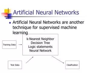
Artificial Neural Networks
E N D
Presentation Transcript
Articifial Intelligence Artificial Neural Networks Brian Talecki CSC 8520 Villanova University
ANN - Artificial Neural Network • A set of algebraic equations and functions which determine the best output given a set of inputs. • An artificial neural network is modeled on a very simplified version of the a human neuron which make up the human nervous system. • Although the brain operates at 1 millionth the speed of modern computers, it functions faster than computers because of the parallel processing structure of the nervous system.
Human Nerve Cell • picture from: G5AIAI Introduction to AIby Graham Kendall • www.cs.nott.ac.uk/~gxk/courses/g5aiai
At the synapse – the nerve cell releases a chemical compounds called neurotransmitters, which excite or inhibit a chemical / electrical discharge in the neighboring nerve cells. • The summation of the responses of the adjacent neurons will elicit the appropriate response in the neuron.
Brief History of ANN • McCulloch and Pitts (1943) designed the first neural network • Hebb (1949) who developed the first learning rule. If two neurons were active at the same time then the strength between them should be increased. • Rosenblatt (1958) – introduced the concept of a perceptron which performed pattern recognition. • Widrow and Hoff (1960) introduced the concept of the ADALINE (ADAptive Linear Element) . The training rule was based on the idea of Least-Mean-Squares learning rule which minimizing the error between the computed output and the desired output. • Minsky and Papert (1969) stated that the perceptron was limited in its ability to recognize features that were separated by linear boundaries. “Neural Net Winter” • Kohonen and Anderson – independently developed neural networks that acted like memories. • Webros(1974) – developed the concept of back propagation of an error to train the weights of the neural network. • McCelland and Rumelhart (1986) published the paper on back propagation algorithm. “Rebirth of neural networks”. • Today - they are everywhere a decision can be made. Source : G5AIAI - Introduction to Artificial Intelligence Graham Kendall:
Inputs – normally a vector of measured parameters Bias – may/may not be added f() – transfer or activation function Outputs = f(∑Wp + b) Basic Neural Network b - Bias ∑ Wp +b f() Inputs ∑ W Outputs T
Activation Functions Source: Supervised Neural Network Introduction CISC 873. Data Mining Yabin Meng
Log Sigmoidal Function Source: Artificial Neural Networks Colin P. Fahey http://www.colinfahey.com/2003apr20_neuron/index.htm
Hard Limit Function y 1.0 x -1.0
Log Sigmoid and Derivative Source : The Scientist and Engineer’s Guide to Digital Signal Processing by Steven Smith
Derivative of the Log Sigmoidal Function s(x) = (1 + e ) s’(x) = -(1+e ) * (-e ) = e * (1+ e ) = ( e ) * ( 1 ) (1+ e ) ( 1 + e ) = (1 + e – 1) * ( 1 ) ( 1+ e ) ( 1 + e ) = (1 - ( 1 ) ) * ( 1 ) (1+ e ) (1 + e ) s’(x) = (1-s(x)) * s(x) -1 -x -2 -x -x -2 -x -x -x -x -x -x -x -x -x -x Derivative is important for the back error propagation algorithm used to train multilayer neural networks.
Given : W = 1.3, p = 2.0, b = 3.0 Wp + b = 1.3(2.0) + 3.0 = 5.6 Linear: f(5.6) = 5.6 Hard limit f(5.6) = 1.0 Log Sigmoidal f(5.6) = 1/(1+exp(-5.6) = 1/(1+0.0037) = .9963 Example : Single Neuron
Simple Neural Network One neuron with a linear activation function => Straight Line Recall the equation of a straight Line : y = mx +b m is the slope (weight), b is the y-intercept (bias). p2 Bad Good Mp1 + b >= p2 Decision Boundary Mp1 + b < p2 p1
Perceptron Learning Extend our simple perceptron to two inputs and hard limit activation function bias W ∑ F() Output p1 W1 Hard limit function p2 W2 o = f (∑ W p + b) W is the weight matrix p is the input vector o is our scalar output T
Rules of Matrix Math Addition/Subtraction 1 2 3 9 8 7 10 10 10 4 5 6 +/- 6 5 4 = 10 10 10 7 8 9 3 2 1 10 10 10 Multiplication by a scalar Transpose a 1 2 = a 2a 1 = 1 2 3 4 3a 4a 2 Matrix Multiplication 2 4 5 = 18 , 5 2 4 = 10 20 2 2 4 8 T
Data Points for the AND Function q1 = 0 , o1 = 0 0 q2 = 1 , o2 = 0 0 q3 = 0 , o3 = 0 1 q4 = 1 , o4 = 1 1 Truth Table P1 P2 O 0 0 0 0 1 0 1 0 0 1 1 1
Weight Vector and the Decision Boundary W = 1.0 1.0 Magnitude and Direction Decision Boundary is the line where W p = b or W p – b = 0 T T As we adjust the weights and biases of the neural network, we change the magnitude and direction of the weight vector or the slope and intercept of the decision boundary T W p > b T W p < b
Perceptron Learning Rule • Adjusting the weights of the Perceptron • Perceptron Error : Difference between the desired and derived outputs. e = Desired – Derived When e = 1 W new = Wold + p When e = -1 W new = Wold - p When e = 0 W new = Wold Simplifing W new = Wold + λ * ep b new = bold + e λ is the learning rate ( = 1 for the perceptron).
AND Function Example Start with W1 = 1, W2 = 1, and b = -1 Wp + b => t - a = e 1 1 0 + -1 => 0 - 0 = 0 N/C 0 1 1 0 + -1 => 0 - 1 = -1 1 1 0 1 + -2 => 0 - 0 = 0 N/C 0 1 0 1 + -2 => 1 - 0 = 1 1 T
T W p + b => t - a = e 2 1 0 + -1 => 0 - 0 = 0 N/C 0 2 1 0 + -1 => 0 - 1 = -1 1 2 0 1 + -2 => 0 - 1 = -1 0 1 0 1 + -3 => 1 - 0 = 1 1
T W p + b => t - a = e 2 1 0 + -2 => 0 - 0 = 0 N/C 0 2 1 0 + -2 => 0 - 0 = 0 N/C 1 2 1 1 + -2 => 0 - 1 = -1 0 1 1 1 + -3 => 1 - 0 = 1 1
T W p + b => t - a = e 2 2 0 + -2 => 0 - 0 = 0 N/C 0 2 2 0 + -2 => 0 - 1 = -1 1 2 1 1 + -3 => 0 - 0 = 0 N/C 0 2 1 1 + -3 => 1 - 1 = 0 N/C 1
T W p + b => t - a = e 2 1 0 + -3 => 0 - 0 = 0 N/C 0 2 1 0 + -3 => 0 - 0 = 0 N/C 1 Done ! 2 p1 Σ f() 1 p2 Hardlim() -3
XOR Function Truth Table X Y Z = (X and not Y) or (not X and Y) 0 0 0 0 1 1 1 0 1 1 1 0 1 0 No single decision boundary can separate the favorable and unfavorable outcomes. x Circuit Diagram y z We will need a more complicated neural net to realize this function
XOR Function – Multilayer Perceptron x W1 Σ f1() W5 W4 b11 W2 b2 f() b12 y Σ W6 W3 f1() z Z = f (W5*f1(W1*x + W4*y+b11) +W6*f1(W2*x + W3*y+b12)+b2) Weights of the neural net are independent of each other, so that we can compute the partial derivatives of z with respect to the weights of the network. i.e. δz / δW1, δz / δW2, δz / δW3, δz / δW4, δz / δW5, δz / δW6
Back Propagation Diagram Neural Networks and Logistic Regression by Lucila Ohno-Machado Decision Systems Group, Brigham and Women’s Hospital, Department of Radiology
Back Propagation Algorithm • This algorithm to train Artificial Neural Networks (ANN) depends to two basic concepts: a) Reduced the Sum Squared Error, SSE, to an acceptable value. b) Reliable data to train your network under your supervision. Simple case : Single input no bias neural net. W1 W2 x z f1 f2 a1 n2 n1 T = desired output
BP Equations n1 = W1 * x a1 = f1(n1) = f1(W1 * x) n2 = W2 * a1 = W2 * f1(n1) = W2 * f1(W1 * x) z = f2(n2) = f2(W2 * f1(W1 * x)) SSE = ½ (z – T) Lets now take the partial derivatives δSSE/ δW2 = (z - T) * δ(z - T)/ δW2 = (z – T) * δz/ δW2 = (z - T) * δf2(n2)/δW2 Chain Rule δf2(n2)/δW2 = (δf2(n2)/δn2)* (δn2/δW2) = (δf2(n2)/δn2)* a1 δSSE/ δW2 = (z - T) * (δf2(n2)/δn2)* a1 Define λto our learning rate (0 < λ< 1, typical λ= 0.2) Compute our new weight: W2(k+1) = W2(k) - λ(δSSE/ δW2) = W2(k) - λ((z - T) * (δf2(n2)/δn2)* a1) 2
Sigmoid function: δf2(n2)/δn2 = f2(n2)(1 – f2(n2)) = z(1 – z) Therefore: W2(k+1) = W2(k) - λ ((z - T) * ( z(1 –z) )* a1) Analysis for W1 n1 = W1 * x a1 = f1(W1*x) n2 = W2 * f1(n1) = W2 * f1(W1 * x) δSSE/ δW1 = (z - T) * δ(z -T )/ δW1 = (z - T) * δz/ δW1 = (z - T) * δf2(n2)/δW1 δf2(n2)/δW1 = (δf2(n2)/δn2)* (δn2/δW1) -> Chain Rule δn2/δW1 = W2 * (δf1(n1)/δW1) = W2 * (δf1(n1)/δn1) * (n1/δW1) -> Chain Rule = W2 * (δf1(n1)/δn1) * x δSSE/ δW1 = (z - T ) * (δf2(n2)/δn2)* W2 * (δf1(n1)/δn1) * x W1(k+1) = W1(k) - λ ((z - T ) * (δf2(n2)/δn2)* W2 * (δf1(n1)/δn1) * x) δf2(n2)/δn2 = z (1 – z) and δf1(n1)/δn1 = a1 ( 1 – a1)
Gradient Descent Error Local minimum Global minimum Training time Neural Networks and Logistic Regression by Lucila Ohno-Machado Decision Systems Group, Brigham and Women’s Hospital, Department of Radiology
2-D Diagram of Gradient Descent Source : Back Propagation algorithm by Olena Lobunets www.essex.ac.uk/ccfea/Courses/ workshops03-04/Workshop4/Workshop%204.ppt
Learning by Example • Training Algorithm: backpropagation of errors using gradient descent training. • Colors: • Red: Current weights • Orange: Updated weights • Black boxes: Inputs and outputs to a neuron • Blue: Sensitivities at each layer Source : A Brief Overview of Neural Networks Rohit Dua, Samuel A. Mulder, Steve E. Watkins, and Donald C. Wunsch campus.umr.edu/smartengineering/ EducationalResources/Neural_Net.ppt
First Pass 0.6225 0.6225 0.6508 0.5 0.5 0.5 0.5 0.5 0.5 0.5 0.5 0.5 0.5 0.6225 0.6225 0.6508 Gradient of the output neuron = slope of the transfer function × error G1= (0.6225)(1-0.6225)(0.0397)(0.5)(2)=0.0093 G2= (0.6508)(1-0.6508)(0.3492)(0.5)=0.0397 0.6508 1 0.6508 G3=(1)(0.3492)=0.3492 Gradient of the neuron= G =slope of the transfer function×[Σ{(weight of the neuron to the next neuron) × (output of the neuron)}] Error=1-0.6508=0.3492
Weight Update 1 New Weight=Old Weight + {(learning rate)(gradient)(prior output)} 0.5+(0.5)(0.0397)(0.6225) 0.5+(0.5)(0.3492)(0.6508) 0.5+(0.5)(0.0093)(1) 0.5124 0.5047 0.6136 0.5124 0.5124 0.5047 0.6136 0.5124 Source : A Brief Overview of Neural Networks Rohit Dua, Samuel A. Mulder, Steve E. Watkins, and Donald C. Wunsch campus.umr.edu/smartengineering/ EducationalResources/Neural_Net.ppt
Second Pass 0.6236 0.6391 0.6545 0.5047 0.5124 0.6136 0.5047 0.5124 0.5124 0.5047 0.6136 0.5047 0.5124 0.6236 0.6391 0.6545 G1= (0.6236)(1-0.6236)(0.5124)(0.0273)(2)=0.0066 G2= (0.6545)(1-0.6545)(0.1967)(0.6136)=0.0273 0.8033 1 0.8033 G3=(1)(0.1967)=0.1967 Source : A Brief Overview of Neural Networks Rohit Dua, Samuel A. Mulder, Steve E. Watkins, and Donald C. Wunsch campus.umr.edu/smartengineering/ EducationalResources/Neural_Net.ppt Error=1-0.8033=0.1967
Weight Update 2 New Weight=Old Weight + {(learning rate)(gradient)(prior output)} 0.5124+(0.5)(0.0273)(0.6236) 0.6136+(0.5)(0.1967)(0.6545) 0.5047+(0.5)(0.0066)(1) 0.5209 0.508 0.6779 0.5209 0.5209 0.508 0.6779 0.5209 Source : A Brief Overview of Neural Networks Rohit Dua, Samuel A. Mulder, Steve E. Watkins, and Donald C. Wunsch campus.umr.edu/smartengineering/ EducationalResources/Neural_Net.ppt
Third Pass 0.6571 0.508 0.508 0.6571 0.6243 0.6504 0.5209 0.8909 0.6779 0.508 1 0.5209 0.5209 0.508 0.6779 0.5209 0.8909 0.6243 0.6504 Source : A Brief Overview of Neural Networks Rohit Dua, Samuel A. Mulder, Steve E. Watkins, and Donald C. Wunsch campus.umr.edu/smartengineering/ EducationalResources/Neural_Net.ppt
Weight Update Summary W1: Weights from the input to the input layer W2: Weights from the input layer to the hidden layer W3: Weights from the hidden layer to the output layer Source : A Brief Overview of Neural Networks Rohit Dua, Samuel A. Mulder, Steve E. Watkins, and Donald C. Wunsch campus.umr.edu/smartengineering/ EducationalResources/Neural_Net.ppt
ECG Interpretation Neural Networks and Logistic Regression by Lucila Ohno-Machado Decision Systems Group, Brigham and Women’s Hospital, Department of Radiology
Other Applications of ANN Lip Reading Using Artificial Neural Network Ahmad Khoshnevis, Sridhar Lavu, Bahar Sadeghi and Yolanda Tsang ELEC502 Course Project www-dsp.rice.edu/~lavu/research/doc/502lavu.ps AI Techniques in Power Electronics and DrivesDr. Marcelo G. Simões Colorado School of Mines egweb.mines.edu/msimoes/tutorial Car Classification with Neural Networks Koichi Sato & Sangho Park hercules.ece.utexas.edu/course/ ee380l/1999sp/present/carclass.ppt Face Detection and Neural Networks Todd Wittman www.ima.umn.edu/~whitman/faces/face_detection2.ppt A Neural Network for Detecting and Diagnosing Tornadic Circulations V Lakshmanan, Gregory Stumpf, Arthur Wittwww.cimms.ou.edu/~lakshman/Papers/mdann_talk.ppt
Bibliography A Brief Overview of Neural Networks Rohit Dua, Samuel A. Mulder, Steve E. Watkins, and Donald C. Wunsch campus.umr.edu/smartengineering/ EducationalResources/Neural_Net.ppt Neural Networks and Logistic Regression Lucila Ohno-Machado Decision Systems Group, Brigham and Women’s Hospital,Department of Radiology dsg.harvard.edu/courses/hst951/ppt/hst951_0320.ppt G5AIAI Introduction to AI by Graham Kendall Schooll of Computer Science and IT , University of Nottingham www.cs.nott.ac.uk/~gxk/courses/g5aiai The Scientist and Engineer's Guide to Digital Signal Processing Steven W. Smith, Ph.D.California Technical Publishing www.dspguide.com Neural Network Design Martin Hagen, Howard B. Demuth, and Mark Beale Campus Publishing Services, Boulder Colorado 80309-0036 ECE 8412 lectures notes by Dr. Anthony Zygmont Department of Electrical Engineering Villanova University January 2003 Supervised Neural Network Introduction CISC 873. Data Mining Yabin Meng meng@cs.queensu.ca