Artificial Neural Networks
Artificial Neural Networks. Dan Simon Cleveland State University. Neural Networks. Artificial Neural Network (ANN) : An information processing paradigm that is inspired by biological neurons

Artificial Neural Networks
E N D
Presentation Transcript
Artificial Neural Networks Dan SimonCleveland State University
Neural Networks • Artificial Neural Network (ANN): An information processing paradigm that is inspired by biological neurons • Distinctive structure: Large number of simple, highly interconnected processing elements (neurons); parallel processing • Inductive learning, that is, learning by example; an ANN is configured for a specific application through a learning process • Learning involves adjustments to connections between the neurons
Inductive Learning • Sometimes we can’t explain how we know something; we rely on our experience • An ANN can generalize from expert knowledge and re-create expert behavior • Example: An ER doctor considers a patient’s age, blood pressure, heart rate, ECG, etc., and makes an educated guess about whether or not the patient had a heart attack
The Birth of ANNs • The first artificial neuron was proposed in 1943 by neurophysiologist Warren McCulloch and the psychologist/logician Walter Pitts • No computing resources at that time
A Simple ANN Pattern recognition: T versus H x11 f1(.) x12 x13 x21 f2(.) g(.) x22 x23 x31 f3(.) x32 x33 1 0
Examples: 1, 1, 1 1 1 0 0, 0, 0 0 1, ? 1 1 0, ?, 1 ? Truth table
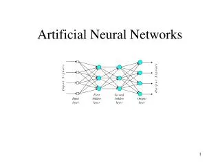
Feedforward ANN How many hidden layers should we use? How many neurons should we use in each hidden layer?
Perceptrons • A simple ANN introduced by Frank Rosenblatt in 1958 • Discredited by Marvin Minsky and Seymour Papert in 1969 • “Perceptrons have been widely publicized as 'pattern recognition' or 'learning machines' and as such have been discussed in a large number of books, journal articles, and voluminous 'reports'. Most of this writing ... is without scientific value …”
Perceptrons x0=1 Three-dimensional single-layer perceptron Problem: Given a set of training data (i.e., (x, y) pairs), find the weight vector {w} that correctly classifies the inputs. w0 x1 w1 w2 x2 w3 x3
The Perceptron Training Rule • t = target output, o = perceptron output • Training rule: wi = e xi, where e = t o,and is the step size.Note that e = 0, 1 or 1.If e = 0, then don’t update the weight.If e = 1, then t = 1 and o = 0, so we need to increase wi if xi > 0, and decrease wi if xi < 0.Similar logic applies when e = 1. • is often initialized to 0.1 and decreases as training progresses.
From Perceptrons to Backpropagation • Perceptrons were dismissed because of: • Limitations of single layer perceptrons • The threshold function is not differentiable • Multi-layer ANNs with differentiable activation functions allow much richer behaviors. A multi-layer perceptron (MLP) is a feedforward ANN with at least one hidden layer.
Backpropagation Derivative-based method for optimizing ANN weights. 1969: First described by Arthur Bryson and Yu-Chi Ho. 1970s-80s: Popularized by David Rumelhart, Geoffrey Hinton Ronald Williams, Paul Werbos; led to a renaissance in ANN research. Derivative-based method for optimizing ANN weights
The Credit Assignment Problem In a multi-layer ANN, how can we tell which weight should be varied to correct an output error? Answer: backpropagation. Output 1 Wanted 0
Backpropagation input neurons hidden neurons output neurons x1 x1 v11 y1 w11 o1 a1 z1 v21 w21 v12 w12 x2 x2 v22 y2 w22 o2 a2 z2 Similar for a2 and y2 Similar for z2 and o2
tk = desired (target) value of k-th output neuron no = number of output neurons Sigmoid transfer function
Hidden Neurons D( j ) = {output neurons whose inputs come from the j-th middle-layer neuron} vij aj yj { zk for all k D( j ) }
The Backpropagation Training Algorithm • Randomly initialize weights {w} and {v}. • Input sample xto get output o. Compute error E. • Compute derivatives of E with respect to output weights {w} (two pages previous). • Compute derivatives of E with respect to hidden weights {v} (previous page). Note that the results of step 3 are used for this computation; hence the term “backpropagation”). • Repeat step 4 for additional hidden layers as needed. • Use gradient descent to update weights {w} and {v}. Go to step 2 for the next sample/iteration.
XOR Example x2 Not linearly separable. This is a very simple problem, but early ANNs were unable to solve it. y = sign(x1x2) 1 0 x1 0 1
XOR Example x1 x1 v11 y1 w11 o1 a1 z1 Bias nodes at both the input and hidden layer w21 v12 v21 y2 w31 x2 x2 v22 a2 v31 v32 1 1 1 1 Backprop.m
XOR Example x2 Homework: Record the weights for the trained ANN, input various (x1, x2) combinations to the ANN to see how well it can generalize. 1 0 x1 0 1
Backpropagation Issues • Momentum: wij wij – jyi + wij,previousWhat value of should we use? • Backpropagation is a local optimizer • Combine it with a global optimizer (e.g., BBO) • Run backprop with multiple initial conditions • Add random noise to input data and/or weights to improve generalization
Backpropagation Issues Batch backpropagation Don’t forget to adjust the learning rate! • Randomly initialize weights {w} and {v} • While not (termination criteria) • For i = 1 to (number of training samples) • Input sample xito get output oi. Compute error Ei • Compute dEi / dw and dEi / dv • Next sample • dE / dw = dEi / dw and dE / dv = dEi / dv • Use gradient descent to update weights {w} and {v}. • End while
Backpropagation Issues Weight decay • wij wij – jyi – dwijThis tends to decrease weight magnitudes unless they are reinforced with backpropd 0.001 • This corresponds to adding a term to the error function that penalizes the weight magnitudes
Backpropagation Issues Quickprop (Scott Fahlman, 1988) • Backpropagation is notoriously slow. • Quickprop has the same philosophy as Newton-Raphson.Assume the error surface is quadratic and jump in one step to the minimum of the quadratic.
Backpropagation Issues • Other activation functions • Sigmoid: f(x) = (1+e–x)–1 • Hyperbolic tangent: f(x) = tanh(x) • Step: f(x) = U(x) • Tan Sigmoid: f(x) = (ecx – e–cx) / (ecx + e–cx) for some positive constant c • How many hidden layers should we use?
Universal Approximation Theorem • A feed-forward ANN with one hidden layer and a finite number of neurons can approximate any continuous function to any desired accuracy. • The ANN activation functions can be any continuous, nonconstant, bounded, monotonically increasing functions. • The desired weights may not be obtainable via backpropagation. • George Cybenko, 1989; Kurt Hornik, 1991
Termination Criterion If we train too long we begin to “memorize” the training data and lose the ability to generalize. Train with a validation/test set. Error Validation/Test Set Training Set
Termination Criterion Cross Validation • N data partitions • N training runs, each using (N1) partitions for training and 1 partition for validation/test • Each training run, store number of epochs cifor the best test set performance (i=1,…,N) • cave = mean{ci} • Train on all data for cave epochs
Adaptive Backpropagation Recall standard weight update: wij wij – jyi • With adaptive learning rates, each weight wij has its own rate ij • If the sign of wij is the same over several backprop updates, then increase ij • If the sign of wij is not the same over several backprop updates, then decrease ij
Double Backpropagation P = number of input training patterns. We want an ANN that can generalize. So input changes should not result in large error changes. In addition to minimizing the training error: Also minimize the sensitivity of training error to input data:
Other ANN Training Methods Gradient-free approaches (GAs, BBO, etc.) • Global optimization • Combination with gradient descent • We can train the structure as well as the weights • We can use non-differentiable activation functions • We can use non-differentiable cost functions BBO.m
Classification Benchmarks The Iris classification problem • 150 data samples • Four input feature values (sepal length and width, and petal length and width) • Three types of irises: Setosa, Versicolour, and Virginica
Classification Benchmarks • The two-spirals classification problem • UC Irvine Machine Learning Repository – http://archive.ics.uci.edu/ml194 benchmarks!
Radial Basis Functions J. Moody and C. Darken, 1989 Universal approximators N middle-layer neurons Inputs x Activation functions f (x, ci) Output weights wik yk = wikf (x, ci) = wik ( ||xci|| ) (.) is a basis function limx ( ||xci|| ) = 0 { ci } are the N RBF centers
Radial Basis Functions Common basis functions: • Gaussian: ( ||xci|| ) = exp(||xci||2 / 2) is the width of the basis function • Many other proposed basis functions
Radial Basis Functions Suppose we have the data set (xi, yi), i = 1, …, N Each xi is multidimensional, each yi is scalar Set ci = xi, i = 1, …, N Define gik = ( || xi xk|| ) Input each xi to the RBF to obtain: Gw = y G is nonsingular if {xi} are distinct Solve for w Global minimum (assuming fixed c and )
Radial Basis Functions We again have the data set (xi, yi), i = 1, …, N Each xi is multidimensional, each yi is scalar ck are given for (k = 1, …, m), and m < N Define gik = ( || xi ck|| ) Input each xi to the RBF to obtain: Gw = y w = (GTG)1GT = G+y
Radial Basis Functions How can we choose the RBF centers? • Randomly select them from the inputs • Use a clustering algorithm • Other options (BBO?) How can we choose the RBF widths?
Other Types of ANNs Many other types of ANNs • Cerebellar Model Articulation Controller (CMAC) • Spiking neural networks • Self-organizing map (SOM) • Recurrent neural network (RNN) • Hopfield network • Boltzman machine • Cascade-Correlation • and many others …
Sources • Neural Networks, by C. Stergiou and D. Siganos, www.doc.ic.ac.uk/~nd/ surprise_96/journal/vol4/cs11/report.html • The Backpropagation Algorithm, by A. Venkataraman, www.speech.sri.com/people/anand/771/html/node37.html • CS 478 Course Notes, by Tony Martinez, http://axon.cs.byu.edu/~martinez

