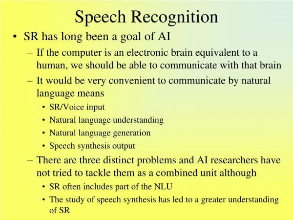
Speech Recognition and Understanding
Speech Recognition and Understanding. Alex Acero Microsoft Research. Thanks to Mazin Rahim (AT&T). “A Vision into the 21 st Century”. Milestones in Speech Recognition . Small Vocabulary, Acoustic Phonetics-based. Large Vocabulary; Syntax, Semantics, .

Speech Recognition and Understanding
E N D
Presentation Transcript
Speech Recognition and Understanding Alex Acero Microsoft Research Thanks to Mazin Rahim (AT&T)
Milestones in Speech Recognition Small Vocabulary, Acoustic Phonetics-based Large Vocabulary; Syntax, Semantics, Very Large Vocabulary; Semantics, Multimodal Dialog Medium Vocabulary, Template-based Large Vocabulary, Statistical-based Isolated Words Connected Digits Continuous Speech Continuous Speech Speech Understanding Spoken dialog; Multiple modalities Connected Words Continuous Speech Isolated Words Stochastic language understanding Finite-state machines Statistical learning Pattern recognition LPC analysis Clustering algorithms Level building Filter-bank analysis Time-normalization Dynamicprogramming Concatenative synthesis Machine learning Mixed-initiative dialog Hidden Markov models Stochastic Language modeling 1962 1967 1972 1977 1982 1987 1992 1997 2003 Year
Multimodal System Technology Components Speech Speech Pen Gesture Visual TTS ASR Automatic SpeechRecognition Text-to-SpeechSynthesis Data, Rules Words Words SLG SLU Spoken Language Generation Spoken LanguageUnderstanding Action Meaning DM DialogManagement
Voice-enabled System Technology Components Speech Speech TTS ASR Automatic SpeechRecognition Text-to-SpeechSynthesis Data, Rules Words Words SLG SLU Spoken Language Generation Spoken LanguageUnderstanding Action Meaning DM DialogManagement
Automatic Speech Recognition • Goal • convert a speech signal into a text message • Accurately and efficiently • independent of the device, speaker or the environment. • Applications • Accessibility • Eyes-busy hands-busy (automobile, doctors, etc) • Call Centers for customer care • Dictation
Basic Formulation • Basic equation of speech recognition is • X=X1,X2,…,Xn is the acoustic observation • is the word sequence. • P(X|W) is the acoustic model • P(W) is the language model
Speech Recognition Process TTS ASR SLG SLU DM Acoustic Model Input Speech Pattern Classification (Decoding, Search) “Hello World” Feature Extraction Confidence Scoring (0.9) (0.8) Word Lexicon Language Model
Acoustic Model Feature Extraction Pattern Classification Confidence Scoring Feature Extraction • Goal: • Extract robust features relevant for ASR • Method: • Spectral analysis • Result: • A feature vector every 10ms • Challenges: • Robustness to environment (office, airport, car) • Devices (speakerphones, cellphones) • Speakers (accents, dialect, style, speaking defects) Language Model Word Lexicon
Spectral Analysis • Female speech (/aa/, pitch of 200Hz) • Fourier transform • 30ms Hamming Window x[n]:time signal X[k]:Fourier transform
Spectrograms • Short-time Fourier transform • Pitch and formant structure
Feature Extraction Process Noise removal, Normalization Quantization Filtering Cepstral Analysis Preemphasis M,N Pitch Formants Spectral Analysis Energy Zero-crossing Segmentation (blocking) Equalization Bias removal or normalization Temporal Derivative Windowing Delta cepstrum Delta^2 cepstrum
Robust Speech Recognition A mismatch in the speech signal between the training phase and testing phase results in performance degradation. Signal Features Model Training Enhancement Normalization Adaptation Signal Features Model Testing
Noise and Channel Distortion y(t) = [s(t) + n(t)] * h(t) Noise n(t) h(t) Channel + Distorted Speech y(t) Speech s(t) 5dB 50dB Fourier Transform Fourier Transform frequency frequency
Speaker Variations • Vocal tract length varies from 15-20cm • Longer vocal tracts =>lower frequency contents • Maximum Likelihood Speaker Normalization • Warp the frequency of a signal
Pattern Classification Confidence Scoring Feature Extraction Acoustic Model Language Model Word Lexicon Acoustic Modeling • Goal: • Map acoustic features into distinct subword units • Such as phones, syllables, words, etc. • Hidden Markov Model (HMM): • Spectral properties modeled by a parametric random process • A collection of HMMs is associated with a subword unit • HMMs are also assigned for modeling extraneous events • Advantages: • Powerful statistical method for a wide range of data and conditions • Highly reliable for recognizing speech
Discrete-Time Markov Process • The Dow Jones Industrial Average Discrete-time first order Markov chain
Example • I observe (up, up, down, up, unchanged, up) • Is it a bull market? bear market? P(bull)=0.7*0.7*0.1*0.7*0.2*0.7*[0.5* (0.6)5]=1.867*10-4 P(bear)=0.1*0.1*0.6*0.1*0.3*0.1*[0.2* (0.3)5]=8.748*10-9 P(steady)=0.3*0.3*0.3*0.3*0.4*0.3*[0.3*(0.5)5]=9.1125*10-6 • It’s 20 times more likely that we are in a bull market than a steady market! • How about P(bull,bull,bear,bull,steady,bull)= =(0.7*0.7*0.6*0.7*0.4*0.7)*(0.5*0.6*0.2*0.5*0.2*0.4)=1.382976*10-4
Basic Problems in HMMs Given acoustic observation X and model: Evaluation: Compute P(X | ) Decoding: Choose optimal state sequence Re-estimation: Adjust to maximize P(X |)
t -2 t+1 t-1 t s1 a1i s1 aj1 Xt aj2 a2i s2 s2 si sj aj3 a3i s3 s3 aijbj(Xt) aNi ajN sN sN bt+1(j) bt(j) t-2(i) t-1(i) Evaluation: Forward-Backward algorithm Forward Backward
Optimal alignment between X and S sM b2(2) Vt-1(j+1) s2 j+1 aj+1 j Vt-1(j) aj j Vt(j) s1 j bj(xt) Vt-1(j-1) aj-1 j j -1 x1 x2 xT t -1 t Decoding: Viterbi Algorithm Step 1: Initialization D1(i)=πibi(x1), B1(i)=0 j=1,…N Step 2: Iterations for t=2,…,T { for j=1,…,N { Vt(j)=min[Vt-1(i)aij ] bj(xt) Bt(j)=argmin[Vt-1(i)aij ] }} Step 3: Backtracking The optimal score is VT = max Vt(i) Final state is sT= argmax Vt(i) Optimal path is (s1,s2,…,sT) where st=Bt+1(st+1) t=T-1,…1
Reestimation:Baum-Welch Algorithm • Find =(A, B, ) that maximize p(X| ): • No closed-form solution => • EM algorithm: • Start with old parameter value • Obtain a new parameter that maximizes • EM guaranteed to have higher likelihood
Continuous Densities • Output distribution is mixture of Gaussians • Posterior probabilities of state j at time t, (mixture k and state i at time t - 1): • Reestimation Formulae:
EM Training Procedure Input speech database Estimate Posteriors t(j,k), t(i,j) Maximize parameters aij, cjk, jk, jk Updated HMM Model Old HMM Model
1 2 0 Design Issues • Continuous vs. Discrete HMM • Whole-word vs. subword (phone units) • Number of states, number of Gaussians • Ergodic vs. Bakis • Context-dependent vs. context-independent a
/sil/ /sil/ one three /sil/ Training with continuous speech • No segmentation is needed • Composed HMM
Context Variability in Speech • At word/sentence level: • Mr. Wright should write to Ms. Wrightright away about his Ford orfour door Honda. • At phone level: /ee/ for words peat and wheel • Triphones capture: • Coarticulation • phonetic context Peat Wheel
Context-dependent models Triphone IY(P, CH) captures coarticulation, phonetic context Stress: Italy vs Italian
Clustering similar triphones • /iy/ with two different left contexts /r/ and /w/ • Similar effects on /iy/ • Cluster those triphones together
Other variability in Speech • Style: • discrete vs. continuous speech, • read vs spontaneous • slow vs fast • Speaker: • speaker independent • speaker dependent • speaker adapted • Environment: • additive noise (cocktail party effect) • telephone channel
Acoustic Adaptation • Model adaptation needed if • Mismatched test conditions • Desire to tune to a given speaker • Maximum a Posteriori (MAP) • adds a prior for the parameters • Maximum Likelihood Linear Regression (MLLR) • Transform mean vectors • Can have more than one MLLR transform • Speaker Adaptive Training (SAT) applies MLLR to training data as well
MAP vs MLLR Speaker-dependent system is trained with 1000 sentences
Discriminative Training • Maximum Likelihood Training: • Parameters obtained from true classes • Discriminative Training: • maximize discrimination between classes Discriminative Feature Transformation • Maximize inter-class difference to intra-class difference • Done at the state level • Linear Discriminant Analysis (LDA) Discriminative Model Training • Maximize posterior probability • Correct class and competing classes are used • Maximum mutual information (MMI); Minimum classification Error (MCE), Minimum Phone Error (MPE)
Acoustic Model Word Lexicon • Goal: • Map legal phone sequences into words • according to phonotactic rules: • David /d/ /ey/ /v/ /ih/ /d/ • Multiple Pronunciation: • Several words may have multiple pronunciations: • Data /d/ /ae/ /t/ /ax/ • Data /d/ /ey/ /t/ /ax/ • Challenges: • How do you generate a word lexicon automatically? • How do you add new variant dialects and word pronunciations? Pattern Classification Confidence Scoring Feature Extraction Language Model Word Lexicon
The Lexicon • An entry per word (> 100K words for dictation) • Multiple pronunciations (tomato) • Done by hand or with letter-to-sound rules (LTS) • LTS rules can be automatically trained with decision trees (CART) • less than 8% errors, but proper nouns are hard!
Acoustic Model Language Model Goal: Model “acceptable” spoken phrases constrained by task syntax Rule-based: Deterministic knowledge-driven grammars: Statistical: Compute estimate of word probabilities (N-gram, class-based, CFG) Pattern Classification Confidence Scoring Feature Extraction Language Model Word Lexicon flying from $cityto $city on $date flying from Newark to Boston tomorrow 0.4 0.6
Ngrams Trigram Estimation
Understanding Bigrams • Training data: • “John read her book” • “I read a different book” • “John read a book by Mark” • But we have a problem here
Ngram Smoothing • Data sparseness: in millions of words more than 50% of trigrams occur only once. • Can’t assign p(wi|wi-1, wi-2)=0 • Solution: assign non-zero probability for each ngram by lowering the probability mass of seen ngrams
Perplexity • Cross-entropy of a language model on word sequence W is • And its perplexity measures the complexity of a language model (geometric mean of branching factor).
Perplexity • For digit recognition task (TIDIGITS) has 10 words, PP=10 and 0.2% error rate • Airline Travel Information System (ATIS) has 2000 words and PP=20 and a 2.5% error rate • Wall Street Journal Task has 5000 words and PP=130 with bigram and 5% error rate • In general, lower perplexity => lower error rate, but it does not take acoustic confusability into account: E-set (B, C, D, E, G, P, T) has PP=7 and has 5% error rate.
Ngram Smoothing • Deleted Interpolation algorithm estimates that maximizes probability on held-out data set • We can also map all out-of-vocabulary words to the unknown word • Other backoff smoothing algorithms possible: Katz, Kneser-Ney, Good-Turing, class ngrams
Adaptive Language Models • Cache Language Models • Topic Language Models • Maximum Entropy Language Models
Bigram Perplexity • Trained on 500 million words and tested on Encarta Encyclopedia
OOV Rate • OOV rate measured on Encarta Encyclopedia. Trained on 500 million words.
WSJ Results • Perplexity and word error rate on the 60000-word Wall Street Journal continuous speech recognition task • Unigrams, bigrams and trigrams were trained from 260 million words • Smoothing mechanisms Kneser-Ney