Speech Recognition
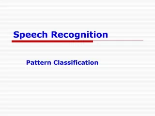
Speech Recognition. Pattern Classification. Pattern Classification. Introduction Parametric classifiers Semi-parametric classifiers Dimensionality reduction Significance testing. Classifier. Feature Extraction. Class i. Feature Vectors x. Observation s. Pattern Classification.


Speech Recognition
E N D
Presentation Transcript
Speech Recognition Pattern Classification
Pattern Classification • Introduction • Parametric classifiers • Semi-parametric classifiers • Dimensionality reduction • Significance testing Veton Këpuska
Classifier Feature Extraction Classi Feature Vectorsx Observations Pattern Classification • Goal: To classify objects (or patterns) into categories (or classes) • Types of Problems: • Supervised: Classes are known beforehand, and data samples of each class are available • Unsupervised: Classes (and/or number of classes) are not known beforehand, and must be inferred from data Veton Këpuska
Probability Basics • Discrete probability mass function (PMF): P(ωi) • Continuous probability density function (PDF): p(x) • Expected value: E(x) Veton Këpuska
Kullback-Liebler Distance • Can be used to compute a distance between two probability mass distributions, P(zi), and Q(zi) • Makes use of inequality log x ≤ x - 1 • Known as relative entropy in information theory • The divergence of P(zi) and Q(zi) is the symmetric sum Veton Këpuska
Bayes Theorem • Define: Veton Këpuska
From Bayes Rule: Where: Bayes Theorem Veton Këpuska
Bayes Decision Theory • The probability of making an error given x is: P(error|x)=1-P(i|x) if decide class i • To minimize P(error|x) (and P(error)): Choose i if P(i|x)>P(j|x) ∀j≠i Veton Këpuska
Bayes Decision Theory • For a two class problem this decision rule means: Choose 1 if else 2 • This rule can be expressed as a likelihood ratio: Veton Këpuska
Bayes Risk • Define cost function λijand conditional risk R(ωi|x): • λijis cost of classifying x as ωiwhen it is really ωj • R(ωi|x) is the risk for classifying x as class ωi • Bayes risk is the minimum risk which can be achieved: • Choose ωiifR(ωi|x) < R(ωj|x) ∀i≠j • Bayes risk corresponds to minimumP(error|x)when • All errors have equal cost (λij = 1, i≠j) • There is no cost for being correct (λii = 0) Veton Këpuska
Discriminant Functions • Alternative formulation of Bayes decision rule • Define a discriminant function, gi(x), for each class ωi Choose ωiif gi(x)>gj(x)∀j ≠i • Functions yielding identical classiffication results: gi(x) = P(ωi|x) = p(x|ωi)P(ωi) = log p(x|ωi)+log P(ωi) • Choice of function impacts computation costs • Discriminant functions partition feature space into decision regions, separated by decision boundaries. Veton Këpuska
Density Estimation • Used to estimate the underlying PDF p(x|ωi) • Parametric methods: • Assume a specific functional form for the PDF • Optimize PDF parameters to fit data • Non-parametric methods: • Determine the form of the PDF from the data • Grow parameter set size with the amount of data • Semi-parametric methods: • Use a general class of functional forms for the PDF • Can vary parameter set independently from data • Use unsupervised methods to estimate parameters Veton Këpuska
Parametric Classifiers • Gaussian distributions • Maximum likelihood (ML) parameter estimation • Multivariate Gaussians • Gaussian classifiers Veton Këpuska
Gaussian Distributions • Gaussian PDF’s are reasonable when a feature vector can be viewed as perturbation around a reference • Simple estimation procedures for model parameters • Classification often reduced to simple distance metrics • Gaussian distributions also called Normal Veton Këpuska
Gaussian Distributions: One Dimension • One-dimensional Gaussian PDF’s can be expressed as: • The PDF is centered around the mean • The spread of the PDF is determined by the variance Veton Këpuska
Maximum Likelihood Parameter Estimation • Maximum likelihood parameter estimation determines an estimate θ for parameter θ by maximizing the likelihoodL(θ) of observing data X = {x1,...,xn} • Assuming independent, identicallydistributed data • ML solutions can often be obtained via the derivative: ^ Veton Këpuska
Maximum Likelihood Parameter Estimation • For Gaussian distributions log L(θ) is easier to solve Veton Këpuska
Gaussian ML Estimation: One Dimension • The maximum likelihood estimate for μ is given by: Veton Këpuska
Gaussian ML Estimation: One Dimension • The maximum likelihood estimate for σ is given by: Veton Këpuska
Gaussian ML Estimation: One Dimension Veton Këpuska
ML Estimation: Alternative Distributions Veton Këpuska
ML Estimation: Alternative Distributions Veton Këpuska
Gaussian Distributions: Multiple Dimensions (Multivariate) • A multi-dimensional Gaussian PDF can be expressed as: • d is the number of dimensions • x={x1,…,xd} is the input vector • μ= E(x)= {μ1,...,μd} is the mean vector • Σ= E((x-μ )(x-μ)t) is the covariance matrix with elements σij, inverse Σ-1 , and determinant |Σ| • σij= σji= E((xi- μi)(xj- μj)) = E(xixj) - μiμj Veton Këpuska
Gaussian Distributions: Multi-Dimensional Properties • If the ithand jthdimensions are statistically or linearly independent then E(xixj)= E(xi)E(xj) and σij=0 • If all dimensions are statistically or linearly independent, then σij=0 ∀i≠j and Σ has non-zero elements only on the diagonal • If the underlying density is Gaussian and Σ is a diagonal matrix, then the dimensions are statistically independent and Veton Këpuska
Diagonal Covariance Matrix:Σ=σ2I Veton Këpuska
Diagonal Covariance Matrix:σij=0 ∀i≠j Veton Këpuska
General Covariance Matrix: σij≠0 Veton Këpuska
Multivariate ML Estimation • The ML estimates for parameters θ = {θ1,...,θl } are determined by maximizing the joint likelihood L(θ) of a set of i.i.d. data x = {x1,..., xn} • To find θ we solve θL(θ)= 0, or θ log L(θ)= 0 • The ML estimates of and are ^ Veton Këpuska
Multivariate Gaussian Classifier • Requires a mean vector i, and a covariance matrix Σifor each of M classes {ω1, ··· ,ωM } • The minimum error discriminant functions are of the form: • Classification can be reduced to simple distance metrics for many situations. Veton Këpuska
Gaussian Classifier: Σi= σ2I • Each class has the same covariance structure: statistically independent dimensions with variance σ2 • The equivalent discriminant functions are: • If each class is equally likely, this is a minimum distance classifier, a form of template matching • The discriminant functions can be replaced by the following linear expression: • where Veton Këpuska
Gaussian Classifier: Σi= σ2I • For distributions with a common covariance structure the decision regions a hyper-planes. Veton Këpuska
Gaussian Classifier: Σi=Σ • Each class has the same covariance structure Σ • The equivalent discriminant functions are: • If each class is equally likely, the minimum error decision rule is the squared Mahalanobis distance • The discriminant functions remain linear expressions: • where Veton Këpuska
Gaussian Classifier: ΣiArbitrary • Each class has a different covariance structure Σi • The equivalent discriminant functions are: • The discriminant functions are inherently quadratic: • where Veton Këpuska
Gaussian Classifier: ΣiArbitrary • For distributions with arbitrary covariance structures the decision regions are defined by hyper-spheres. Veton Këpuska
3 Class Classification (Atal & Rabiner, 1976) • Distinguish between silence, unvoiced, and voiced sounds • Use 5 features: • Zero crossing count • Log energy • Normalized first autocorrelation coefficient • First predictor coefficient, and • Normalized prediction error • Multivariate Gaussian classifier, ML estimation • Decision by squared Mahalanobis distance • Trained on four speakers (2 sentences/speaker), tested on 2 speakers (1 sentence/speaker) Veton Këpuska
Maximum A Posteriori Parameter Estimation • Bayesian estimation approaches assume the form of the PDF p(x|θ) is known, but the value of θ is not • Knowledge of θ is contained in: • An initial a priori PDF p(θ) • A set of i.i.d. data X = {x1,...,xn} • The desired PDF for xis of the form • The value posteriori θ that maximizes p(θ|X) is called the maximum a posteriori (MAP) estimate of θ ^ Veton Këpuska
Gaussian MAP Estimation: One Dimension • For a Gaussian distribution with unknown mean μ: • MAP estimates of μand x are given by • As n increases, p(μ|X) converges to μ, and p(x,X) converges to the ML estimate ~ N(μ,2) ^ ^ Veton Këpuska
References • Huang, Acero, and Hon, Spoken Language Processing, Prentice-Hall, 2001. • Duda, Hart and Stork, Pattern Classification, John Wiley & Sons, 2001. • Atal and Rabiner, A Pattern Recognition Approach to Voiced-Unvoiced-Silence Classification with Applications to Speech Recognition, IEEE Trans ASSP, 24(3), 1976. Veton Këpuska