Introduction to Machine Learning
Introduction to Machine Learning. Paulos Charonyktakis Maria Plakia. Roadmap. Supervised Learning Algorithms Artificial Neural Networks Naïve Bayes Classifier Decision Trees Application on VoIP in Wireless Networks. Machine Learning.

Introduction to Machine Learning
E N D
Presentation Transcript
Introduction to Machine Learning • Paulos Charonyktakis • Maria Plakia
Roadmap • Supervised Learning • Algorithms • Artificial Neural Networks • Naïve Bayes Classifier • Decision Trees • Application on VoIP in Wireless Networks
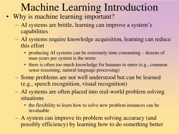
Machine Learning • The study of algorithms and systems that improve their performance with experience (Mitchell book) • Experience? • Experience = data / measurements / observations
Where to Use Machine Learning • You have past data, you want to predict the future • You have data, you want to make sense out of them (find useful patterns) • You have a problem it’s hard to find an algorithm for • Gather some input-output pairs, learn the mapping • Measurements + intelligent behavior usually lead to some form of Machine Learning
Supervised Learning • Learn from examples • Would like to be able to predict an outcome of interest y for an object x • Learn function y = f(x) • For example, x is a VoIP call, y is an indicator of QoE • We are given data with pairs {<xi, yi> : i=1, ..., n}, • xi the representation of an object • yi the representation of a known outcome • Learn the function y = f(x) that generalizes from the data the “best” (has minimum average error)
Algorithms: Artificial Neural Networks
Binary Classification Example • The simplest non-trivial decision function is the straight line (in general a hyperplane) • One decision surface • Decision surface partitions space into two subspaces
Specifying a Line Line equation: • Classifier: • If • Output 1 • Else • Output -1
Classifying with Linear Surfaces • Classifier becomes
Training Perceptrons • Start with random weights • Update in an intelligent way to improve them using the data • Intuitively: • Decrease the weights that increase the sum • Increase the weights that decrease the sum • Repeat for all training instances until convergence
PerceptronTraining Rule • η: arbitrary learning rate (e.g. 0.5) • td: (true) label of the dth example • od: output of the perceptron on the dth example • xi,d: value of predictor variable i of example d • td= od : No change (for correctly classified examples)
Analysis of the Perceptron Training Rule • Algorithm will always converge within finite number of iterations if the data are linearly separable. • Otherwise, it may oscillate (no convergence)
Training by Gradient Descent • Similar but: • Always converges • Generalizes to training networks of perceptrons (neural networks) and training networks for multicategory classification or regression • Idea: • Define an error function • Search for weights that minimize the error, i.e., find weights that zero the error gradient
Use Differentiable Transfer Functions • Replace with the sigmoid
Updating the Weights with Gradient Descent • Each weight update goes through all training instances • Each weight update more expensive but more accurate • Always converges to a local minimum regardless of the data • When using the sigmoid: output is a real number between 0 and 1 • Thus, labels (desired outputs) have to be represented with numbers from 0 to 1
From the Viewpoint of the Output Layer • Each hidden layer maps to a new feature space • •Each hidden node is a new constructed feature • •Original Problem may become separable (or easier)
How to Train Multi-Layered Networks • Select a network structure (number of hidden layers, hidden nodes, and connectivity). • Select transfer functions that are differentiable. • Define a (differentiable) error function. • Search for weights that minimize the error function, using gradient descent or other optimization method. • BACKPROPAGATION
Back-Propagation Algorithm • Propagate the input forward through the network • Calculate the outputs of all nodes (hidden and output) • Propagate the error backward • Update the weights:
Training with Back-Propagation • Going once through all training examples and updating the weights: one epoch • Iterate until a stopping criterion is satisfied • The hidden layers learn new features and map to new spaces • Training reaches a local minimum of the error surface
Overfittingwith Neural Networks • If number of hidden units (and weights) is large, it is easy to memorize the training set (or parts of it) and not generalize • Typically, the optimal number of hidden units is much smaller than the input units • Each hidden layer maps to a space of smaller dimension
Representational Power • Perceptron: Can learn only linearly separable functions • Boolean Functions: learnable by a NN with one hidden layer • Continuous Functions: learnable with a NN with one hidden layer and sigmoid units • Arbitrary Functions: learnable with a NN with two hidden layers and sigmoid units • Number of hidden units in all cases unknown
Conclusions • Can deal with both real and discrete domains • Can also perform density or probability estimation • Very fast classification time • Relatively slow training time (does not easily scale to thousands of inputs) • One of the most successful classifiers yet • Successful design choices still a black art • Easy to overfit or underfit if care is not applied
ANN in Matlab • Create an ANN net =feedforwardnet(hiddenSizes,trainFcn) • [NET,TR] = train(NET,X,T) takes a network NET, input data X and target data T and returns the network after training it, and a training record TR. • sim(NET,X) takes a network NET and inputs X and returns the estimated outputs Y generated by the network.
Bayes Classifier • Training data: • Learning = estimating P(X|Y), P(Y) • Classification = using Bayes rule to calculate P(Y | Xnew)
Naïve Bayes • Naïve Bayes assumes X= <X1, …, Xn >, Y discrete-valued • i.e., that Xi and Xj are conditionally independent given Y, for all i≠j
Conditional Independence • Definition: X is conditionally independent of Y given Z, if the probability distribution governing X is independent of the value of Y, given the value of Z • P(X| Y, Z) = P(X| Z)
Naïve Bayes • Naïve Bayes uses assumption that the Xi are conditionally independent, given Y then: How many parameters need to be calculated???
Naïve Bayes classification • Bayes rule: • Assuming conditional independence: • So, classification rule for Xnew = <Xi, …, Xn>
Naïve Bayes Algorithm • Train Naïve Bayes (examples) • for each* value yk • Estimate πk = P(Y = yk) • for each* value xij of each attribute Xi • Estimate θijk = P(Xi = xij| Y = yk) • Classify (Xnew) * parameters must sum to 1
Estimating Parameters: Y, Xi discrete-valued • Maximum likelihood estimates: • MAP estimates (uniform Dirichlet priors):
What if we have continuous Xi ? • Gaussian Naïve Bayes (GNB) assume Sometimes assume variance • is independent of Y (i.e., σi), • or independent of Xi (i.e., σk) • or both (i.e., σ)
Estimating Parameters: Y discrete, Xi continuous • Maximum likelihood estimates:
Naïve Bayes in Matlab • Create a new Naïve object: NB = NaiveBayes.fit(X, Y), X is a matrix of predictor values, Y is a vector of n response values • post = posterior(nb,test) returns the posterior probability of the observations in test • Predict a value predictedValue= predict(NB,TEST)