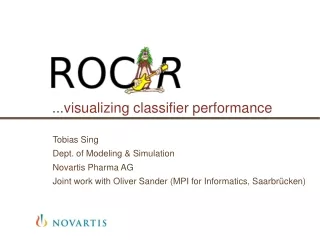
...visualizing classifier performance
...visualizing classifier performance. Tobias Sing Dept. of Modeling & Simulation Novartis Pharma AG Joint work with Oliver Sander (MPI for Informatics, Saarbr ü cken). Classification. Binary classification (Instances, Class labels): (x 1 , y 1 ), (x 2 , y 2 ), ..., (x n , y n )


...visualizing classifier performance
E N D
Presentation Transcript
...visualizing classifier performance Tobias Sing Dept. of Modeling & Simulation Novartis Pharma AG Joint work with Oliver Sander (MPI for Informatics, Saarbrücken)
Classification • Binary classification • (Instances, Class labels): (x1, y1), (x2, y2), ..., (xn, yn) • yi {1,-1} - valued • Classifier: provides class prediction Ŷ for an instance • Outcomes for a prediction: True class Predictedclass 2 | ROCR | Tobias Sing | July 2, 2007
Some basic performance measures • P(Ŷ = Y): accuracy • P(Ŷ = 1 | Y = 1): true positive rate • P(Ŷ = 1 | Y = -1): false positive rate • P(Y = 1 | Ŷ = 1): precision True class Predictedclass 3 | ROCR | Tobias Sing | July 2, 2007
Performance trade-offs • Often: Improvement in measure X measure Y becomes worse • Idea: Visualize trade-off in a two-dimensional plot • Examples: • True pos. rate vs.false pos. rate • Precision vs. recall • Lift charts • … 4 | ROCR | Tobias Sing | July 2, 2007
Scoring classifiers • Output: continuous(instead of actualclass prediction) • Discretized by choosinga cut-off • f(x) ≥ c class „1“ • f(x) < c class „-1“ • Trade-off visualizations:cutoff-parameterized curves 5 | ROCR | Tobias Sing | July 2, 2007
ROCR • Only three commands • pred <- prediction( scores, labels )(pred: S4 object of class prediction) • perf <- performance( pred, measure.Y, measure.X)(pred: S4 object of class performance) • plot( perf ) • Input format • Single run:vectors (scores: numeric; labels: anything) • Multiple runs (cross-validation, bootstrapping, …): matrices or lists 6 | ROCR | Tobias Sing | July 2, 2007
Examples (1/8): ROC curves • pred <- prediction(scores, labels) • perf <- performance(pred, "tpr", "fpr") • plot(perf, colorize=T) 7 | ROCR | Tobias Sing | July 2, 2007
Examples (2/8): Precision/recall curves • pred <- prediction(scores, labels) • perf <- performance(pred, "prec", "rec") • plot(perf, colorize=T) 8 | ROCR | Tobias Sing | July 2, 2007
Examples (3/8): Averaging across multiple runs • pred <- prediction(scores, labels) • perf <- performance(pred, "tpr", "fpr") • plot(perf, avg='threshold', spread.estimate='stddev', colorize=T) 9 | ROCR | Tobias Sing | July 2, 2007
Examples (4/8): Performance vs. cutoff • perf <- performance(pred, "cal", window.size=50) • plot(perf) • perf <- performance(pred, "acc") • plot(perf, avg= "vertical", spread.estimate="boxplot", show.spread.at= seq(0.1, 0.9, by=0.1)) 10 | ROCR | Tobias Sing | July 2, 2007
Examples (5/8): Cutoff labeling • pred <- prediction(scores, labels) • perf <- performance(pred,"pcmiss","lift") • plot(perf, colorize=T, print.cutoffs.at=seq(0,1,by=0.1), text.adj=c(1.2,1.2), avg="threshold", lwd=3) 11 | ROCR | Tobias Sing | July 2, 2007
Examples (6/8): Cutoff labeling – multiple runs • plot(perf,print.cutoffs.at=seq(0,1,by=0.2),text.cex=0.8,text.y=lapply(as.list(seq(0,0.5,by=0.05)), function(x) { rep(x,length(perf@x.values[[1]]))}),col= as.list(terrain.colors(10)),text.col= as.list(terrain.colors(10)),points.col= as.list(terrain.colors(10))) 12 | ROCR | Tobias Sing | July 2, 2007
Examples (7/8): More complex trade-offs... • perf <- performance(pred,"acc","lift") • plot(perf, colorize=T) • plot(perf, colorize=T, print.cutoffs.at=seq(0,1,by=0.1), add=T, text.adj=c(1.2, 1.2), avg="threshold", lwd=3) 13 | ROCR | Tobias Sing | July 2, 2007
Examples (8/8): Some other examples • perf<-performance( pred, 'ecost') • plot(perf) • perf<-performance( pred, 'rch') • plot(perf) 14 | ROCR | Tobias Sing | July 2, 2007
Extending ROCR: An example • Extend environments • assign("auc", "Area under the ROC curve",envir = long.unit.names) • assign("auc", ".performance.auc",envir = function.names) • assign("auc", "fpr.stop", envir=optional.arguments) • assign("auc:fpr.stop", 1, envir=default.values) • Implement performance measure (predefined signature) • .performance.auc <- function (predictions, labels, cutoffs, fp, tp, fn,tn, n.pos, n.neg, n.pos.pred, n.neg.pred, fpr.stop){} 15 | ROCR | Tobias Sing | July 2, 2007
Thank you! • http://rocr.bioinf.mpi-sb.mpg.de • Sing et al. (2005) Bioinformatics 16 | ROCR | Tobias Sing | July 2, 2007