Bayesian Classifier

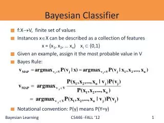
1. Bayesian Classifier • f:XV, finite set of values • Instances xX can be described as a collection of features x = (x1, x2, … xn) xi2 {0,1} • Given an example, assign it the most probable value in V • Bayes Rule: • Notational convention: P(y) means P(Y=y)

2. Bayesian Classifier VMAP = argmaxvP(x1, x2, …, xn | v )P(v) • Given training data we can estimate the two terms. • Estimating P(v) is easy. For each value v count how many times it appears in the training data. • However, it is not feasible to estimate P(x1, x2, …, xn | v ) • In this case we have to estimate, for each target value, the probability of each instance (most of which will not occur). • In order to use a Bayesian classifiers in practice, we need to make assumptions that will allow us to estimate these quantities.

3. Naive Bayes VMAP = argmaxvP(x1, x2, …, xn | v )P(v) • Assumption: feature values are independent given the target value

4. Naive Bayes (2) VMAP = argmaxvP(x1, x2, …, xn | v )P(v) • Assumption: feature values are independent given the target value P(x1 = b1, x2 = b2,…,xn = bn| v = vj ) = ¦1n P(xn = bn| v = vj) • Generative model: • First choose a value vjV according to P(v) • For each vj: choose x1 x2, …, xnaccording to P(xk |vj)

5. Naive Bayes (3) VMAP = argmaxvP(x1, x2, …, xn | v )P(v) • Assumption: feature values are independent given the target value P(x1 = b1, x2 = b2,…,xn = bn| v = vj ) = ¦1nP(xi= bi | v = vj) • Learning method: Estimate n|V| + |V| parameters and use them to make a prediction. (How to estimate?) • Notice that this is learning without search. Given a collection of training examples, you just compute the best hypothesis (given the assumptions). • This is learning without trying to achieve consistency or even approximate consistency. • Why does it work?

6. Conditional Independence • Notice that the features values are conditionallyindependent • given the target value, and are not required to be independent. • Example:The features are x and y. • We define the label to be l = f(x,y)=xy • over the product distribution: p(x=0)=p(x=1)=1/2 and p(y=0)=p(y=1)=1/2 • The distribution is defined so that x and y areindependent: p(x,y) = p(x)p(y) • That is: • But, given that l =0: • p(x=1| l =0) = p(y=1| l =0) = 1/3 • while: p(x=1,y=1 | l =0) = 0 • so x and y are not conditionally independent.

7. Conditional Independence • The other direction also does not hold. • x and y can be conditionally independent but not independent. • Example: We define a distribution s.t.: • l =0: p(x=1| l =0) =1, p(y=1| l =0) = 0 • l =1: p(x=1| l =1) =0, p(y=1| l =1) = 1 • and assume, that: p(l =0) = p(l =1)=1/2 • Giventhe value of l, x and y are independent(check) • What about unconditional independence ? • p(x=1) = p(x=1| l =0)p(l =0)+p(x=1| l =1)p(l =1) = 0.5+0=0.5 • p(y=1) = p(y=1| l =0)p(l =0)+p(y=1| l =1)p(l =1) = 0+0.5=0.5 • But, • p(x=1, y=1)=p(x=1,y=1| l =0)p(l =0)+p(x=1,y=1| l =1)p(l =1) = 0 • so x and y are not independent.

8. Example Day Outlook Temperature Humidity WindPlayTennis 1 Sunny Hot High Weak No 2 Sunny Hot High Strong No 3 Overcast Hot High Weak Yes 4 Rain Mild High Weak Yes 5 Rain Cool Normal Weak Yes 6 Rain Cool Normal Strong No 7 Overcast Cool Normal Strong Yes 8 Sunny Mild High Weak No 9 Sunny Cool Normal Weak Yes 10 Rain Mild Normal Weak Yes 11 Sunny Mild Normal Strong Yes 12 Overcast Mild High Strong Yes 13 Overcast Hot Normal Weak Yes 14 Rain Mild High Strong No

9. Estimating Probabilities • How do we estimate ?

10. Example • Compute P(PlayTennis= yes); P(PlayTennis= no) • Compute P(outlook= s/oc/r | PlayTennis= yes/no)(6 numbers) • Compute P(Temp= h/mild/cool | PlayTennis= yes/no)(6 numbers) • Compute P(humidity= hi/nor | PlayTennis= yes/no)(4 numbers) • Compute P(wind= w/st | PlayTennis= yes/no)(4 numbers)

11. Example • Compute P(PlayTennis= yes); P(PlayTennis= no) • Compute P(outlook= s/oc/r | PlayTennis= yes/no)(6 numbers) • Compute P(Temp= h/mild/cool | PlayTennis= yes/no)(6 numbers) • Compute P(humidity= hi/nor | PlayTennis= yes/no)(4 numbers) • Compute P(wind= w/st | PlayTennis= yes/no)(4 numbers) • Given a new instance: • (Outlook=sunny; Temperature=cool; Humidity=high; Wind=strong) • Predict:PlayTennis= ?

12. Example • Given: (Outlook=sunny; Temperature=cool; Humidity=high; Wind=strong) • P(PlayTennis= yes)=9/14=0.64 P(PlayTennis= no)=5/14=0.36 • P(outlook = sunny | yes)= 2/9 P(outlook = sunny | no)= 3/5 • P(temp = cool | yes) = 3/9 P(temp = cool | no) = 1/5 • P(humidity = hi |yes) = 3/9 P(humidity = hi | no) = 4/5 • P(wind = strong | yes) = 3/9 P(wind = strong | no)= 3/5 • P(yes, …..) ~ 0.0053 P(no, …..) ~ 0.0206

13. Example • Given: (Outlook=sunny; Temperature=cool; Humidity=high; Wind=strong) • P(PlayTennis= yes)=9/14=0.64 P(PlayTennis= no)=5/14=0.36 • P(outlook = sunny | yes)= 2/9 P(outlook = sunny | no)= 3/5 • P(temp = cool | yes) = 3/9 P(temp = cool | no) = 1/5 • P(humidity = hi |yes) = 3/9 P(humidity = hi | no) = 4/5 • P(wind = strong | yes) = 3/9 P(wind = strong | no)= 3/5 • P(yes, …..) ~ 0.0053 P(no, …..) ~ 0.0206 • P(no|instance) = 0.0206/(0.0053+0.0206)=0.795 • What if we were asked about Outlook=OC ?

14. Estimating Probabilities • How do we estimate ? • Sparsity of data is a problem • -- if is small, the estimate is not accurate • -- if is 0, it will dominate the estimate: we will never predict • if a word that never appeared in training (with ) • appears in the test data

15. Robust Estimation of Probabilities • This process is called smoothing. • There are many ways to do it, some better justified than others; • An empirical issue. • Here: • nk is # of occurrences of the word in the presence of v • n is # of occurrences of the label v • p is a prior estimate of v (e.g., uniform) • m is equivalent sample size(# of labels)

16. Robust Estimation of Probabilities Smoothing: Common values: Laplace Rule: for the Boolean case, p=1/2 , m=2 Learn to classify text: p = 1/(|values|) (uniform) m= |values|

17. Naïve Bayes: Two Classes • Notice that the naïve Bayes method gives a method for predicting • rather than an explicit classifier. • In the case of two classes, v{0,1} we predict that v=1 iff:

18. Naïve Bayes: Two Classes • Notice that the naïve Bayes method gives a method for predicting • rather than an explicit classifier. • In the case of two classes, v{0,1} we predict that v=1 iff:

19. Naïve Bayes: Two Classes • In the case of two classes, v{0,1} we predict that v=1 iff:

20. Naïve Bayes: Two Classes • In the case of two classes, v{0,1} we predict that v=1 iff:

21. Naïve Bayes: Two Classes • In the case of two classes, v{0,1} we predict that v=1iff: • We get that naive Bayes is a linear separator with

22. Naïve Bayes: Two Classes • In the case of two classes we have that: • but since • We get: • Which is simply the logistic function (used also in the neural network • representation). • The linearity of NB provides a better explanation for why it works. We have: A = 1-B; Log(B/A) = -C. Then: Exp(-C) = B/A = = (1-A)/A = 1/A – 1 = + Exp(-C) = 1/A A = 1/(1+Exp(-C))

23. Example: Learning to Classify Text • Instance space X: Text documents • Instances are labeled according to f(x)=like/dislike • Goal: Learn this function such that, given a new document • you can use it to decide if you like it or not • How to represent the document ? • How to estimate the probabilities ? • How to classify?

24. Document Representation • Instance space X: Text documents • Instances are labeled according to y = f(x) = like/dislike • How to represent the document ? • A document will be represented as a list of its words • The representation question can be viewed as the generation question • We have a dictionary of n words (therefore 2n parameters) • We have documents of size N: can account for word position& count • Having a parameter for each word & position may be too much: • # of parameters: 2 x Nx n (2 x 100 x 50,000 ~ 107) • Simplifying Assumption: • The probability of observing a word in a document is independent of its location • This still allows us to think about two ways of generating the document

25. Classification via Bayes Rule (B) • We want to compute • argmaxyP(y|D) = argmaxy P(D|y) P(y)/P(D) = • = argmaxy P(D|y)P(y) • Our assumptions will go into estimating P(D|y): • Multivariate Bernoulli • To generate a document, first decide if it’s good(y=1) or bad (y=0). • Given that, consider your dictionary of words and choose w into your document with probability p(w |y), irrespective of anything else. • If the size of the dictionaryis |V|=n, we can then write • P(d|y) = ¦1n P(wi=1|y)bi P(wi=0|y)1-bi • Where: • p(w=1/0|y): the probability that w appears/does-not in a y-labeled document. • bi {0,1} indicates whether word wioccurs in document d • 2n+2 parameters: • Estimating P(wi =1|y) and P(y)is done in the ML way as before (counting). Parameters: Priors: P(y=0/1) 8wi2Dictionary p(wi =0/1 |y=0/1)

26. A Multinomial Model • We want to compute • argmaxyP(y|D) = argmaxy P(D|y) P(y)/P(D) = • = argmaxy P(D|y)P(y) • Our assumptions will go into estimating P(D|y): • 2. Multinomial • To generate a document, first decide if it’s good(y=1) or bad (y=0). • Given that, place N words into d, such that wi is placed with probability P(wi|y), andiNP(wi|y) =1. • The Probability of a document is: • P(d|y) N!/n1!...nk! P(w1|y)n1…p(wk|y)nk • Where niis the # of times wi appears in the document. • Same # of parameters: 2n+2, where n = |Dictionary|, but the estimation is done a bit differently. (HW). Parameters: Priors: P(y=0/1) 8wi2Dictionary p(wi =0/1 |y=0/1) N dictionary items are chosen into D

27. Model Representation • The generative model in these two cases is different µ ¯ µ ¯ label label Documents d Appear Documents d Appear (d) Position p Words w Bernoulli: A binary variable corresponds to a document d and a dictionary word w, and it takes the value 1 if w appears in d. Document topic is governed by a prior µ, its topic (label), and the variable in the intersection of the plates is governed by µ and the Bernoulli parameter ¯ for the dictionary word w Multinomial: Words do not correspond to dictionary words but to positions (occurrences) in the document d. The internal variable is then W(D,P). These variables are generated from the same multinomial distribution ¯, and depend on the topic.

28. General NB Scenario • We assume a mixture probability model, parameterized by µ. • Different components {c1,c2,… ck} of the model are parameterize by disjoint subsets of µ. • The generative story: A document d is created by • (1) selecting a component according to the priors, P(cj |µ), then • (2) having the mixture component generate a document according to its own parameters, with distribution P(d|cj, µ) • So we have: • P(d|µ) = 1k P(cj|µ) P(d|cj,µ) • In the case of document classification, we assume a one to one correspondence between components and labels.

29. Naïve Bayes: Continuous Features • Xi can be continuous • We can still use • And

30. Naïve Bayes: Continuous Features • Xi can be continuous • We can still use • And • Naïve Bayes classifier:

31. Naïve Bayes: Continuous Features • Xi can be continuous • We can still use • And • Naïve Bayes classifier: • Assumption: P(Xi|Y) has a Gaussian distribution

32. The Gaussian Probability Distribution • Gaussian probability distribution also called normal distribution. • It is a continuous distribution = mean of distribution • 2 = variance of distribution • x is a continuous variable (-∞x∞ • Probability of x being in the range [a, b]cannot be evaluated analytically (has to be looked up in a table) x

33. Naïve Bayes: Continuous Features • P(Xi|Y) is Gaussian • Training: estimate mean and standard deviation Note that the following slides abuse notation significantly. Since P(x) =0 for continues distributions, we think of P (X=x| Y=y), not as a classic probability distribution, but just as a function f(x) = N(x, ¹, ¾2). f(x) behaves as a probability distribution in the sense that 8x, f(x) ¸ 0 and the values add up to 1. Also, note that f(x) satisfies Bayes Rule, that is, it is true that: fY(y|X = x) = fX (x|Y = y) fY (y)/fX(x)

34. Naïve Bayes: Continuous Features • P(Xi|Y) is Gaussian • Training: estimate mean and standard deviation X1 X2 X3 Y 2 3 1 1 -1.2 2 .4 1 2 0.3 0 0 2.2 1.1 0 1

35. Naïve Bayes: Continuous Features • P(Xi|Y) is Gaussian • Training: estimate mean and standard deviation X1 X2 X3 Y 2 3 1 1 -1.2 2 .4 1 2 0.3 0 0 2.2 1.1 0 1

36. Recall: Naïve Bayes, Two Classes • In the case of two classes we have that: • but since • We get: • Which is simply the logistic function(also used in the neural network • representation) • The same formula can be written for continuous features

37. Logistic Function: Continuous Features • Logistic function for Gaussian features Note that we are using ratio of probabilities, since x is a continuous variable.