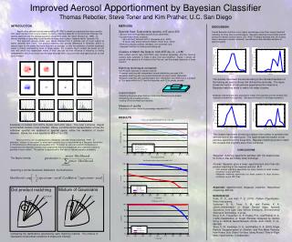
Enhanced Aerosol Apportionment Algorithm Utilizing Bayesian Classifier
This research presents an improved method for apportioning ambient aerosol particles using a Bayesian classifier. The approach addresses limitations of current methods by considering cluster size and variability in spectra. Experimental data from ATOFMS is used to compare different matching techniques, including dot product and Bayesian methods for cluster classification. The study shows that Bayesian matching offers better accuracy in particle apportionment compared to traditional dot product matching. The results demonstrate the effectiveness of the Bayesian classifier in reducing apportionment errors and biases in cluster assignments.

Enhanced Aerosol Apportionment Algorithm Utilizing Bayesian Classifier
E N D
Presentation Transcript
Improved Aerosol Apportionment by Bayesian Classifier Thomas Rebotier, Steve Toner and Kim Prather, U.C. San Diego Α=arcos(V.F.) Seed2 Seed3 Seed1 Mixture of Gaussians Dot product matching S.Dx Seed2 Seed3 Seed1 INTRODUCTION Apportioning ambient aerosol measured by ATOFMS is made by comparing their mass spectra with seeds obtained from source studies. Currently, matching depends on the dot product between the particle spectrum and the average spectrum of a particle class, the “seed” (Song et al., 1999). An aerosol matches a class when its dot product is larger than a given “vigilance factor” (typically 0.8). This approach ignores cluster size: seeds obtained from 5 particles pull as much weight as seeds obtained from 2,000. Dot product matching also ignores differences in variability: Δ(m/z) is always larger for the peaks that have large m/z on average, so that the existence of smaller significant peaks is entirely swamped by noise on larger peaks. For example, Na2Cl creates two peaks (at +81 and +83) which very dependable marks of fresh sea salt but their influence in matching is nothing compared to that of the noise from the large Na peak which occurs in fresh and aged sea salt, as well as in biomass. • METHODS • Spectral Data: Dual polarity spectra, m/Z up to 350 • Aerosol Time-Of-Flight Mass Spectrometer (ATOFMS) • Dynamometer Study: originally: • 28 Light Duty Vehicles (LDVs) (Sodeman et al., 2005) • 6 Heavy Duty Diesel Vehicles (HDDV) (Toner et al., 2005) • Removing atypical vehicles (smokers, non-converter cars) • Separate Vehicles for training and testing set. • Clusters to Match the Data to: from ART-2a, v.f. = 0.85 • Each subset vehicle type (LDV/HDV) was clustered separately, and the resulting clusters were collected, to make 2 sets: Fine and UltraFine. Figure 1 shows the spread of the spectra for 8 clusters in the Fine set, and the median spectrum of these clusters. • Matching techniques compared: • Dot Product matching to nearest centroid • Bayesian matching with independent normal distribution per peak (Full) • Bayesian matching with one normal distribution for each cluster (Spherical) • Bayesian matching with quartile-based “box" distribution (the likelihood is a product of 1 for peaks within the 2nd and third quartiles and 0.5 for peaks outside) • Useful Details: • Adjusting the priors when classes come from different source studies • Simplifying the covariance matrix • Cutting off the low likelihood matches • Measure of quality: • Percentage correct related to percentage matched (R.O.C.) DISCUSSION: Overall Bayesian matching has a higher percentage correct than nearest centroid matching, but they have opposite biases. Bayesian matching favors HDVs and dot product to nearest centroid favors LDV. Why? Probably because the LDV clusters have in average a smaller “diameter” (as defined by their standard deviation in spectral space). The clusters have been binned according to the standard deviation of the training set spectra (those that defined the centroids). The figure shows the fraction of test particles apportioned into these bins. Bayesian matching tends to match into wider clusters. Bayesian matching was also expected to match more particles into the clusters that originally included more particles. (Because of the prior in the Bayes equation). RESULTS Examples of clusters from HDVs (trucks) and LDVs (cars). The most numerous, largest and smallest clusters of are included. Above, a 2-dimensional representation of how the individual spectral are scattered in spectral space; notice the variations of cluster diameter. Below, the mass spectra for M/Z=+1 to +100. The clusters have been binned according to the number of particles that defined them in the training set. The figure shows the fraction of test particles apportioned into these bins. Bayesian matching tends to match into clusters that originally were more numerous. These problems can be addressed by a Bayesian Classifier (Duda and Heart, 1973). In particular, “mixture of Gaussians” in which each spectral class is represented by a Gaussian distribution in 700 dimensions (350 positive and negative m/z). To match an unknown particle, its likelihood is computed by the Gaussian formula, then weighted by the prior probabilities (the expected number of particles in each cluster). The particle is apportioned to the class of highest posterior probability. • CONCLUSIONS • Bayesian matching apportions particles with the desired bias for clusters that are initially wider and larger • Overall, Bayesian gives a lower apportionment error than dot product matching to the nearest centroid. BUT • Dot product matching apportions too many spectra to small clusters, resulting in a pro-LDV bias • Bayesian matching apportions too many spectra to large clusters, resulting in a pro-HDV bias. • Keywords: Apportionment, Bayesian Classifier, Hierarchical Clustering, ART-2A • REFERENCES • Duda, R. O., and Hart, P. E. (1973). Pattern Classification, Wiley Interscience. • Sodeman, D. A., Toner, S. M., and Prather, K. A. (2005).Determination of Single Particle Mass Spectral Signatures from Light Duty Vehicle Emissions, Environmental Science & Technology, in press. • Song, X.-H., Fergenson, D. P., Hopke, P. K., and Prather, K. A. (1999).Classification of Single Particles Analyzed by Atofms Using an Artificial Neural Network, Art-2a, Anal. Chem, 71 (4), 860-865. • Toner, S. M., Sodeman, D. A., and Prather, K. A. (2005).Single Particle Characterization of Ultrafine- and Fine-Mode Particles from Heavy Duty Diesel Vehicles Using Aerosol Time-of-Flight Mass Spectrometry, in preparation. The Bayes formula: Assuming a normal (Gaussian) distribution, the likelihood is: Comparing the distributions assumed by each matching method. The mixture of Gaussians model allows variations of shape and intensity.