Robust Estimation Methods for Population Parameters
290 likes | 451 Vues
Explore sufficiency, unbiasedness, efficiency, and resistance in estimating population parameters using M-estimators and trimmed mean for non-normal data. Learn to overcome challenges in communication and variance heterogeneity.

Robust Estimation Methods for Population Parameters
E N D
Presentation Transcript
The Robust Approach Dealing with real data
Estimating Population Parameters • Four properties are considered desirable in a population estimator: • Sufficiency • Unbiasedness • Efficiency • Resistance
Sampling Distribution • In order to examine the properties of a statistic we often want to take repeated samples from some population of data and calculate the relevant statistic on each sample. • We can then look at the distribution of the statistic across these samples and ask a variety of questions about it.
Properties of a Statistic • Sufficiency • A sufficient statistic is one that makes use of all of the information in the sample to estimate its corresponding parameter • For example, this property makes the mean more attractive as a measure of central tendency compared to the mode or median. • Unbiasedness • A statistic is said to be an unbiased estimator if its expected value (i.e., the mean of a number of sample means) is equal to the population parameter it is estimating. • As one can see using the resampling procedure, the mean can be shown to be an unbiased estimator
Properties of a Statistic • Efficiency • The efficiency of a statistic is reflected in the variance that is observed when one examines the statistic over independently chosen samples • Standard error • The smaller the variance, the more efficient the statistic is said to be • Resistance • The resistance of an estimator refers to the degree to which that estimate is effected by extreme values i.e. outliers • Small changes in the data result in only small changes in estimate • Finite-sample breakdown point • Measure of resistance to contamination • The smallest proportion of observations that, when altered sufficiently, can render the statistic arbitrarily large or small • Median = n/2 • Trimmed mean = whatever the trimming amount is • Mean = 1/n
The Problems • Nonnormality • Arbitrarily small departures from normality can have tremendous influence on mean and variance estimates, resulting in: • Low power • Underestimated effect size • Inability to accurately assess correlation • Problematic inference
The problems • Heterogeneity of variances • Among groups it leads to low power and biased results • In the heteroscedastic situation in regression, bias may even be worse
The problems • Communication • Those that know about the problem and have for some time (statisticians) have been unable to get their findings to the larger audience of applied researchers • Standard methods still dominate, and who knows how many findings have been lost (type II error) or found (type I error) due to problematic data
Measures of Central Tendency • What we want: • A statistic whose standard error will not be grossly affected with small departures from normality • Power to be comparable to that of mean and sd when dealing with a normal population • The value to be fairly stable when dealing with non-normal distributions • Two classes to speak of: • Trimmed mean • M-estimators
Trimmed mean • You are very familiar with this in terms of the median, in which essentially all but the middle value is trimmed • But now we want to retain as much of the data for best performance but enough to ensure resistance to outliers • How much to trim? • About 20%, and that means from both sides • Example: 15 values. .2 * 15 = 3, remove 3 largest and 3 smallest
Trimmed mean • How does it perform? • In non-normal situations it will perform better than the mean • We already know it will be resistant to outliers • It will have a reduced standard error as well
Trimmed mean • How does it perform? • Under normal situations about as well as the mean • Slightly less efficient • With a symmetric population the mean, median, trimmed mean etc. values will be the same • But the population becomes skewed, the mean is much more affected
Trimmed mean • It may be difficult at first to get used to the idea of trimming your data • One way to start getting over it is to ask yourself if you ever had a problem with the median as a measure of location • However, the gains in using the trimmed mean (accuracy of inference, resistance, efficiency) have been shown to offset the sufficiency loss • What you might also consider is: • Do you, when conducting analyses qualify your inferences in terms of generalizing to outliers specifically? Or do you think of it as applying to the groups in general?
M-estimators • M-estimators are another robust measure of location • Involves the notion of a ‘loss function’ • Examples: • If we want to minimize squared errors from a particular value the result of the measure of central tendency will be the mean • If we want to minimize absolute errors, the result will be a median • M-estimators are more mathematically complex, but we can get the gist in that less weight is given to values that are further away from ‘center’ • Different M-Estimators give different weights for deviating values
M-estimators • Wilcox example with more detail, to show the ‘gist’ of the calculation • Data = 3,4,8,16,24,53 • We will start by using a measure of outlierness as follows • What it means: • M = median • MAD = median absolute deviation • Order deviations from the median, pick the median of those outliers • .6745 = dividing by this allows this measure of variance to equal the population standard deviation • When we do will call it MADN • So basically it’s the old ‘Z score > x’ approach just made resistant to outliers
M-estimators • Median = 12 • Median absolute deviation • -9 -8 -4 4 12 41 4 4 8 9 12 41 • MAD is 8.5, 8.5/.6745 = 12.6 • So if the absolute deviation from the median divided by 12.6 is greater than 1.28, we will call it an outlier • In this case the value of 53 is an outlier • (53-12)/12.6 = 3.25
M-estimators • L = number of outliers less than the median • For our data none qualify • U = number of outliers greater than the median • For our data 1 value is an upper outlier • B = sum of values that are not outliers • Notice that if there are no outliers, this would default to the mean
M-estimators • Pretty much the same as the trimmed mean when normal or non-normal • However either might be more accurate in some situations, best to compare both • And as with the trimmed mean, it will outperform the mean if there are outliers
Inferential use of robust statistics • In general, the approach will be the same using robust statistics as we have with regular ones as far as hypothesis testing and interval estimation • Of particular concern will be estimating the standard error and the relative merits of the robust approach
The Trimmed Mean • Consider the typical t-statistic for the one sample case • This will hold using a trimmed mean as well, except we will be using the remaining values after trimming and our inference will regard the population trimmed mean instead of the population mean
The Trimmed Mean • The problem is calculating the standard error • When using the trimmed mean, its properties mean that we do not have independent values in the calculation of the standard error due to the ordering of observations, the result of which is introducing bias into the calculation • Our ‘area under the curve’ no longer would equal 1 • The gist is that in order to get around this problem we will winsorize, rather than trim, in calculating the standard error
Example: Winsorized Mean 1 2 2 2 3 3 3 3 3 3 4 4 4 4 4 5 5 6 8 10 3 3 3 3 3 3 3 3 3 3 4 4 4 4 4 5 5 5 5 5 • Make some percentage of the most extreme values the same as the previous, non-extreme value • Think of the 20% Winsorized mean as affecting the same number of values as the trimming • = 3.75 in this example • Mean = 3.95
Trimmed mean • So what we do is windsorize the data to calculate the standard error, and this will solve our technical issues • We would calculate the CIs in the same fashion as always, just dealing with the trimmed situation. • To determine the df and thus critical value, subtract 2*number of values trimmed from the regular n-1 degrees of freedom
Trimmed means • The two sample case • Here again, the concept remains the same
Trimmed means • Calculating the variance for the group one mean • h refers to the n remaining after trimming • Do the same for group 2 *Note that this formulation works for unequal sample sizes also
Trimmed means • While these approaches work well for dealing with normally distributed data, as mentioned the typical t approach is unsatisfactory when dealing with non-normal data • Use the bootstrap approaches as described previously
M-estimators • We can make inferences using M-estimators as well • While we’d like to do the same with M-estimators, it really can’t be done outside of the bootstrap approach • In particular, use the percentile bootstrap (as opposed to the percentile t) approach and do your hypothesis testing with confidence intervals
Effect size • As Cohen’s d is a sample statistic, use the appropriate data for the trimmed case • Calculate Cohen’s d with the non-trimmed values (trimmed means and winsorized variance/sd) • With M-estimators the general approach remains in effect as well
Summary • Given the issues regarding means, variances and inferences based on them, a robust approach is appropriate and preferred when dealing with outliers/non-normal data • Increased power • More accurate assessment of group tendencies and differences • More accurate assessment of effect size • If we want the best estimates and best inference given not-so-normal situations, standard methods simply don’t work too well • We now have the methods and computing capacity to take a more robust approach to data analysis, and should not be afraid to use them.